নোট

এই পৃষ্ঠাটি docs/tutorials/10_qgan_option_pricing.ipynb থেকে নেয়া হয়েছে।

qGANs দিয়ে বিকল্প মূল্য নির্ধারণ

ভূমিকা

এখন আমরা আলোচনা করব কোয়ান্টাম জেনারেটিভ অ্যাডভারসারিয়াল নেটওয়ার্ক (qGAN) নামে একটি কোয়ান্টাম মেশিন লার্নিং ধারাক্রম (অ্যালগরিদম)। এর একটি ব্যবহারিক প্রয়োগ দেখানো হবে যেখানে qGAN ব্যবহার করে একটি কোয়ান্টাম সার্কিট মডেল করা হবে যা ইউরোপিয়ান কল অপশনের মূল্য নির্ধারন করতে পারবে। এই মডেলটিকে কোয়ান্টাম বিস্তার এস্টিমেশন এলগোরিদম দ্বারা যাচাই করা যাবে, যা থেকে গড় মূল্যের মান নির্ণয় করা যাবে। বিস্তারিত জানতে European Call Option Pricing এই নোটবুক ফাইল ব্যবহারের অনুরোধ রইল। একটি qGAN প্রশিক্ষণ দিয়ে দৈব বণ্টন শেখার এবং লোড করার বিষয়ে আরও বিস্তারিত জানার জন্য অনুগ্রহ করে এই সহায়িকা গবেষণাপত্রটি পড়ুন Quantum Generative Adversarial Networks for Learning and Loading Random Distributions. Zoufal, Lucchi, Woerner. 2019.

import matplotlib.pyplot as plt
import numpy as np

from qiskit.circuit import ParameterVector
from qiskit.circuit.library import TwoLocal
from qiskit.quantum_info import Statevector

from qiskit_algorithms import IterativeAmplitudeEstimation, EstimationProblem
from qiskit_aer.primitives import Sampler
from qiskit_finance.applications.estimation import EuropeanCallPricing
from qiskit_finance.circuit.library import NormalDistribution

অনিশ্চয়তা মডেল

ব্ল্যাক-স্কোলস মডেল অনুমান করে যে পরিপক্কতার সময় স্পট মূল্য \(S_T\) একটি ইউরোপীয় কল বিকল্পের জন্য log-normally distributed হয়। এইভাবে, আমরা একটি লগ-নরমাল ডিস্ট্রিবিউশন থেকে নমুনার উপর একটি qGAN প্রশিক্ষণ দিতে পারি এবং ফলাফলটিকে একটি অনিশ্চয়তা মডেল হিসেবে ব্যবহার করতে পারি। নিম্নলিখিতগুলিতে, আমরা একটি কোয়ান্টাম সার্কিট তৈরি করি যা অনিশ্চয়তা মডেল লোড করে। সার্কিট আউটপুটটি এইটা পড়ে

\[\big| g_{\theta}\rangle = \sum_{j=0}^{2^n-1}\sqrt{p_{\theta}^{j}} \big| j \rangle ,\]

যেখানে সম্ভাব্যতা \(p_{\theta}^{j}\), for \(j\in \left\{0, \ldots, {2^n-1} \right\}\), একটি লক্ষ্য বণ্টনের (টার্গেট ডিস্ট্রিবিউশন) মডেল প্রতিনিধিত্ব করে।

# Set upper and lower data values
bounds = np.array([0.0, 7.0])
# Set number of qubits used in the uncertainty model
num_qubits = 3

# Load the trained circuit parameters
g_params = [0.29399714, 0.38853322, 0.9557694, 0.07245791, 6.02626428, 0.13537225]

# Set an initial state for the generator circuit
init_dist = NormalDistribution(num_qubits, mu=1.0, sigma=1.0, bounds=bounds)

# construct the variational form
var_form = TwoLocal(num_qubits, "ry", "cz", entanglement="circular", reps=1)

# keep a list of the parameters so we can associate them to the list of numerical values
# (otherwise we need a dictionary)
theta = var_form.ordered_parameters

# compose the generator circuit, this is the circuit loading the uncertainty model
g_circuit = init_dist.compose(var_form)

গড় বেতন মূল্য নির্ধারণ কর

Now, the trained uncertainty model can be used to evaluate the expectation value of the option’s payoff function with Quantum Amplitude Estimation.

# set the strike price (should be within the low and the high value of the uncertainty)
strike_price = 2

# set the approximation scaling for the payoff function
c_approx = 0.25

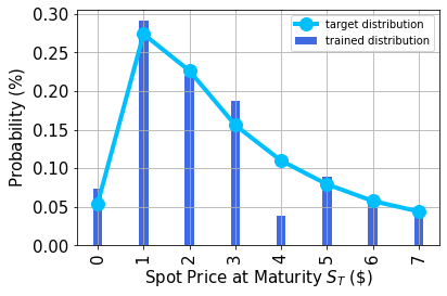
সম্ভাব্যতা বণ্টনের লেখচিত্র অঙ্কন কর

তারপর, আমরা প্রশিক্ষিত (ট্রেইনড) সম্ভাব্যতা বিস্তারের লেখচিত্র এবং তুলনা করার জন্য লক্ষ্য (টার্গেট) সম্ভাব্যতা বিস্তারের লেখচিত্রটিও অঙ্কন করি।

# Evaluate trained probability distribution
values = [
    bounds[0] + (bounds[1] - bounds[0]) * x / (2**num_qubits - 1) for x in range(2**num_qubits)
]
uncertainty_model = g_circuit.assign_parameters(dict(zip(theta, g_params)))
amplitudes = Statevector.from_instruction(uncertainty_model).data

x = np.array(values)
y = np.abs(amplitudes) ** 2

# Sample from target probability distribution
N = 100000
log_normal = np.random.lognormal(mean=1, sigma=1, size=N)
log_normal = np.round(log_normal)
log_normal = log_normal[log_normal <= 7]
log_normal_samples = []
for i in range(8):
    log_normal_samples += [np.sum(log_normal == i)]
log_normal_samples = np.array(log_normal_samples / sum(log_normal_samples))

# Plot distributions
plt.bar(x, y, width=0.2, label="trained distribution", color="royalblue")
plt.xticks(x, size=15, rotation=90)
plt.yticks(size=15)
plt.grid()
plt.xlabel("Spot Price at Maturity $S_T$ (\$)", size=15)
plt.ylabel("Probability ($\%$)", size=15)
plt.plot(
    log_normal_samples,
    "-o",
    color="deepskyblue",
    label="target distribution",
    linewidth=4,
    markersize=12,
)
plt.legend(loc="best")
plt.show()

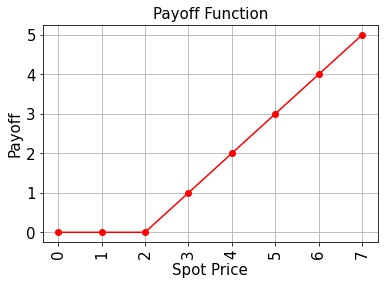
গড় বেতন মূল্য নির্ধারণ কর

Now, the trained uncertainty model can be used to evaluate the expectation value of the option’s payoff function analytically and with Quantum Amplitude Estimation.

# Evaluate payoff for different distributions
payoff = np.array([0, 0, 0, 1, 2, 3, 4, 5])
ep = np.dot(log_normal_samples, payoff)
print("Analytically calculated expected payoff w.r.t. the target distribution:  %.4f" % ep)
ep_trained = np.dot(y, payoff)
print("Analytically calculated expected payoff w.r.t. the trained distribution: %.4f" % ep_trained)

# Plot exact payoff function (evaluated on the grid of the trained uncertainty model)
x = np.array(values)
y_strike = np.maximum(0, x - strike_price)
plt.plot(x, y_strike, "ro-")
plt.grid()
plt.title("Payoff Function", size=15)
plt.xlabel("Spot Price", size=15)
plt.ylabel("Payoff", size=15)
plt.xticks(x, size=15, rotation=90)
plt.yticks(size=15)
plt.show()

Analytically calculated expected payoff w.r.t. the target distribution:  1.0611
Analytically calculated expected payoff w.r.t. the trained distribution: 0.9805

# construct circuit for payoff function
european_call_pricing = EuropeanCallPricing(
    num_qubits,
    strike_price=strike_price,
    rescaling_factor=c_approx,
    bounds=bounds,
    uncertainty_model=uncertainty_model,
)

# set target precision and confidence level
epsilon = 0.01
alpha = 0.05

problem = european_call_pricing.to_estimation_problem()
# construct amplitude estimation
ae = IterativeAmplitudeEstimation(
    epsilon_target=epsilon, alpha=alpha, sampler=Sampler(run_options={"shots": 100, "seed": 75})
)

result = ae.estimate(problem)

conf_int = np.array(result.confidence_interval_processed)
print("Exact value:        \t%.4f" % ep_trained)
print("Estimated value:    \t%.4f" % (result.estimation_processed))
print("Confidence interval:\t[%.4f, %.4f]" % tuple(conf_int))

Exact value:            0.9805
Estimated value:        1.0138
Confidence interval:    [0.9883, 1.0394]

import qiskit.tools.jupyter

%qiskit_version_table
%qiskit_copyright

Version Information

Software	Version
qiskit	None
qiskit-terra	0.45.0.dev0+c626be7
qiskit_algorithms	0.2.0
qiskit_aer	0.12.0
qiskit_optimization	0.6.0
qiskit_finance	0.4.0
qiskit_ibm_provider	0.6.1
System information
Python version	3.9.7
Python compiler	GCC 7.5.0
Python build	default, Sep 16 2021 13:09:58
OS	Linux
CPUs	2
Memory (Gb)	5.778430938720703
Fri Aug 18 16:26:01 2023 EDT

This code is a part of Qiskit

© Copyright IBM 2017, 2023.

This code is licensed under the Apache License, Version 2.0. You may
obtain a copy of this license in the LICENSE.txt file in the root directory
of this source tree or at http://www.apache.org/licenses/LICENSE-2.0.

Any modifications or derivative works of this code must retain this
copyright notice, and modified files need to carry a notice indicating
that they have been altered from the originals.