নোট
এই পৃষ্ঠাটি docs/tutorials/08_fixed_income_pricing.ipynb থেকে নেয়া হয়েছে।
Pricing Fixed-Income Assets (নির্দিষ্ট আয় সম্পদ মূল্য নির্ধারণ)#
ভূমিকা#
প্রাসঙ্গিক সুদের হারগুলি বর্ণনা করে এমন বিতরণগুলি জেনে আমরা একটি নির্দিষ্ট-আয়ের সম্পদের মূল্য চাই। সম্পদের নগদ \(c_t\) প্রবাহ এবং যে তারিখে তারা ঘটে সেগুলি জানা যায়। সম্পত্তির মোট মূল্য \(V\) হল এর গড় মান:
প্রতিটি নগদ প্রবাহকে শূন্য কুপন বন্ড হিসেবে বিবেচনা করা হয় যার সাথে সংশ্লিষ্ট সুদের হার \(r_t\) যা তার পরিপক্কতার উপর নির্ভর করে। ব্যবহারকারীকে অবশ্যই প্রতিটি \(r_t\) (সম্ভবত পারস্পরিক সম্পর্কযুক্ত) অনিশ্চয়তার বণ্টন মডেলিং নির্দিষ্ট করতে হবে এবং সেইসাথে প্রতিটি বন্টনের নমুনার জন্য তিনি যে কিউবিটগুলি ব্যবহার করতে চান তা উল্লেখ করতে হবে। এই উদাহরণে আমরা সম্পদের মান সুদের হারে প্রথম অর্ডারে প্রসারিত করি \(r_t\)। এটি সম্পদের সময়কাল অনুসারে অধ্যয়নের সাথে মিলে যায়। উদ্দেশ্য ফাংশনের আনুমানিকতা নিম্নলিখিত গবেষণা অনুসরণ করে: Quantum Risk Analysis. Woerner, Egger. 2018.
[1]:
import matplotlib.pyplot as plt

%matplotlib inline
import numpy as np
from qiskit import QuantumCircuit
from qiskit_algorithms import IterativeAmplitudeEstimation, EstimationProblem
from qiskit_aer.primitives import Sampler
from qiskit_finance.circuit.library import NormalDistribution
অনিশ্চয়তা মডেল#
We construct a circuit to load a multivariate normal random distribution in \(d\) dimensions into a quantum state. The distribution is truncated to a given box \(\otimes_{i=1}^d [low_i, high_i]\) and discretized using \(2^{n_i}\) grid points, where \(n_i\) denotes the number of qubits used for dimension \(i = 1,\ldots, d\). The unitary operator corresponding to the circuit implements the following:
যেখানে \(p_{i_1, ..., i_d}\) সংক্ষিপ্ত এবং বিযুক্ত বিতরণগুলির সম্ভাবনা বোঝায় এবং \(i_j\) অ্যাফাইন ম্যাপ ব্যবহার করে \([low_j, high_j]\) ডান বিরতি ব্যবধানে ম্যাপ করা হয়েছে:
In addition to the uncertainty model, we can also apply an affine map, e.g. resulting from a principal component analysis. The interest rates used are then given by:
যেখানে \(\vec{x} \in \otimes_{i=1}^d [low_i, high_i]\) প্রদত্ত দৈব (random) বণ্টন অনুসরণ করে।
[2]:
# can be used in case a principal component analysis has been done to derive the uncertainty model, ignored in this example.
A = np.eye(2)
b = np.zeros(2)

# specify the number of qubits that are used to represent the different dimenions of the uncertainty model
num_qubits = [2, 2]

# specify the lower and upper bounds for the different dimension
low = [0, 0]
high = [0.12, 0.24]
mu = [0.12, 0.24]
sigma = 0.01 * np.eye(2)

# construct corresponding distribution
bounds = list(zip(low, high))
u = NormalDistribution(num_qubits, mu, sigma, bounds)
[3]:
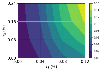
# plot contour of probability density function
x = np.linspace(low[0], high[0], 2 ** num_qubits[0])
y = np.linspace(low[1], high[1], 2 ** num_qubits[1])
z = u.probabilities.reshape(2 ** num_qubits[0], 2 ** num_qubits[1])
plt.contourf(x, y, z)
plt.xticks(x, size=15)
plt.yticks(y, size=15)
plt.grid()
plt.xlabel("$r_1$ (%)", size=15)
plt.ylabel("$r_2$ (%)", size=15)
plt.colorbar()
plt.show()
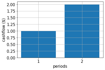
নগদ প্রবাহ, পে-অফ ফাংশন এবং সঠিক গড় মান#
নিম্নলিখিত অংশটিতে আমরা সময়কালে নগদ প্রবাহ সংজ্ঞায়িত করি, ফলাফলের পে-অফ ফাংশন এবং সঠিক গড় মানটি মূল্যায়ন করি।
পে-অফ ফাংশনের জন্য আমরা প্রথমে, প্রথম অর্ডার অনুমান ব্যবহার করি এবং তারপরে European Call Option এর পে-অফ ফাংশনের রৈখিক অংশের মতো একই আনুমানিক পদ্ধতি প্রয়োগ করি।
[4]:
# specify cash flow
cf = [1.0, 2.0]
periods = range(1, len(cf) + 1)

# plot cash flow
plt.bar(periods, cf)
plt.xticks(periods, size=15)
plt.yticks(size=15)
plt.grid()
plt.xlabel("periods", size=15)
plt.ylabel("cashflow ($)", size=15)
plt.show()
[5]:
# estimate real value
cnt = 0
exact_value = 0.0
for x1 in np.linspace(low[0], high[0], pow(2, num_qubits[0])):
    for x2 in np.linspace(low[1], high[1], pow(2, num_qubits[1])):
        prob = u.probabilities[cnt]
        for t in range(len(cf)):
            # evaluate linear approximation of real value w.r.t. interest rates
            exact_value += prob * (
                cf[t] / pow(1 + b[t], t + 1)
                - (t + 1) * cf[t] * np.dot(A[:, t], np.asarray([x1, x2])) / pow(1 + b[t], t + 2)
            )
        cnt += 1
print("Exact value:    \t%.4f" % exact_value)
Exact value: 2.1942
[6]:
# specify approximation factor
c_approx = 0.125

# create fixed income pricing application
from qiskit_finance.applications.estimation import FixedIncomePricing

fixed_income = FixedIncomePricing(
    num_qubits=num_qubits,
    pca_matrix=A,
    initial_interests=b,
    cash_flow=cf,
    rescaling_factor=c_approx,
    bounds=bounds,
    uncertainty_model=u,
)
[7]:
fixed_income._objective.draw()
[7]:
     ┌────┐
q_0: ┤0   ├
     │    │
q_1: ┤1   ├
     │    │
q_2: ┤2 F ├
     │    │
q_3: ┤3   ├
     │    │
q_4: ┤4   ├
     └────┘
[8]:
fixed_income_circ = QuantumCircuit(fixed_income._objective.num_qubits)

# load probability distribution
fixed_income_circ.append(u, range(u.num_qubits))

# apply function
fixed_income_circ.append(fixed_income._objective, range(fixed_income._objective.num_qubits))

fixed_income_circ.draw()
[8]:
     ┌───────┐┌────┐
q_0: ┤0      ├┤0   ├
     │       ││    │
q_1: ┤1      ├┤1   ├
     │  P(X) ││    │
q_2: ┤2      ├┤2 F ├
     │       ││    │
q_3: ┤3      ├┤3   ├
     └───────┘│    │
q_4: ─────────┤4   ├
              └────┘
[9]:
# set target precision and confidence level
epsilon = 0.01
alpha = 0.05

# construct amplitude estimation
problem = fixed_income.to_estimation_problem()

ae = IterativeAmplitudeEstimation(
    epsilon_target=epsilon, alpha=alpha, sampler=Sampler(run_options={"shots": 100, "seed": 75})
)
[10]:
result = ae.estimate(problem)
[11]:
conf_int = np.array(result.confidence_interval_processed)
print("Exact value:        \t%.4f" % exact_value)
print("Estimated value:    \t%.4f" % (fixed_income.interpret(result)))
print("Confidence interval:\t[%.4f, %.4f]" % tuple(conf_int))
Exact value:            2.1942
Estimated value:        2.3437
Confidence interval:    [2.3101, 2.3772]
[12]:
import qiskit.tools.jupyter

%qiskit_version_table
%qiskit_copyright
Version Information
| Software | Version |
|---|---|
qiskit | None |
qiskit-terra | 0.45.0.dev0+c626be7 |
qiskit_finance | 0.4.0 |
qiskit_algorithms | 0.2.0 |
qiskit_ibm_provider | 0.6.1 |
qiskit_optimization | 0.6.0 |
qiskit_aer | 0.12.0 |
| System information | |
| Python version | 3.9.7 |
| Python compiler | GCC 7.5.0 |
| Python build | default, Sep 16 2021 13:09:58 |
| OS | Linux |
| CPUs | 2 |
| Memory (Gb) | 5.778430938720703 |
| Fri Aug 18 16:21:18 2023 EDT | |
This code is a part of Qiskit
© Copyright IBM 2017, 2023.
This code is licensed under the Apache License, Version 2.0. You may
obtain a copy of this license in the LICENSE.txt file in the root directory
of this source tree or at http://www.apache.org/licenses/LICENSE-2.0.
Any modifications or derivative works of this code must retain this
copyright notice, and modified files need to carry a notice indicating
that they have been altered from the originals.
[ ]: