নোট
এই পৃষ্ঠাটি docs/tutorials/01_portfolio_optimization.ipynb -থেকে বানানো হয়েছে।
পোর্টফোলিও অপটিমাইজেশন#
ভূমিকা#
এই টিউটোরিয়াল দেখায় কীভাবে \(n\) সম্পদের জন্য নীচের মীন-ভ্যারিয়্যান্স পোর্টফোলিও অপ্টিমাইজেশান সমস্যাটি সমাধান করা যায়:
যেখানে আমরা নিম্নলিখিত স্বরলিপি ব্যবহার করি:
\(x \in \{0, 1\}^n\) বাইনারি সিদ্ধান্ত ভেরিয়েবলের ভেক্টরকে বোঝায়, যা কোন সম্পদ বাছাই করে তা নির্দেশ করে (\(x[i] = 1\)) এবং কোনটি বেছে নেবে না (\(x[i] = 0\)),
\(\mu \in \mathbb{R}^n\) সম্পদের প্রত্যাশিত রিটার্ন সংজ্ঞায়িত করে,
\(\Sigma \in \mathbb{R}^{n \times n}\) সম্পদের মধ্যে সমবায়িকাগুলি নির্দিষ্ট করে,
\(q > 0\) সিদ্ধান্ত গ্রহণকারীর ঝুঁকি ক্ষুধা নিয়ন্ত্রণ করে,
and \(B\) denotes the budget, i.e. the number of assets to be selected out of \(n\).
We assume the following simplifications: - all assets have the same price (normalized to 1), - the full budget \(B\) has to be spent, i.e. one has to select exactly \(B\) assets.
The equality constraint \(1^T x = B\) is mapped to a penalty term \((1^T x - B)^2\) which is scaled by a parameter and subtracted from the objective function. The resulting problem can be mapped to a Hamiltonian whose ground state corresponds to the optimal solution. This notebook shows how to use the Sampling Variational Quantum Eigensolver (SamplingVQE) or the Quantum Approximate Optimization Algorithm (QAOA) from Qiskit
Algorithms to find the optimal solution for a given set of parameters.
Experiments on real quantum hardware for this problem are reported for instance in the following paper: Improving Variational Quantum Optimization using CVaR. Barkoutsos et al. 2019.
[1]:
from qiskit.circuit.library import TwoLocal
from qiskit.result import QuasiDistribution
from qiskit_aer.primitives import Sampler
from qiskit_algorithms import NumPyMinimumEigensolver, QAOA, SamplingVQE
from qiskit_algorithms.optimizers import COBYLA
from qiskit_finance.applications.optimization import PortfolioOptimization
from qiskit_finance.data_providers import RandomDataProvider
from qiskit_optimization.algorithms import MinimumEigenOptimizer
import numpy as np
import matplotlib.pyplot as plt
import datetime
সমস্যা দৃষ্টান্ত (ইনস্ট্যান্স) সংজ্ঞায়িত করুন#
আমাদের হ্যামিলটনীয়ানের জন্য এখানে একটি অপারেটর উদাহরণ তৈরি করা হয়েছে। এক্ষেত্রে পলিসগুলি পোর্টফোলিও সমস্যা থেকে অনূদিত আইসিং হ্যামিলটোনিয়ান থেকে এসেছে। এই নোটবুকের জন্য আমরা একটি এলোমেলো পোর্টফোলিও সমস্যা ব্যবহার করি। বাস্তব অর্থনৈতিক ডাটা ব্যবহার করে একে বিস্তৃত করা বেশ সোজা-সাপ্টা, যেমনটা দেখানো হয়েছে এখানটায়: Loading and Processing Stock-Market Time-Series Data
[2]:
# set number of assets (= number of qubits)
num_assets = 4
seed = 123

# Generate expected return and covariance matrix from (random) time-series
stocks = [("TICKER%s" % i) for i in range(num_assets)]
data = RandomDataProvider(
    tickers=stocks,
    start=datetime.datetime(2016, 1, 1),
    end=datetime.datetime(2016, 1, 30),
    seed=seed,
)
data.run()
mu = data.get_period_return_mean_vector()
sigma = data.get_period_return_covariance_matrix()
[3]:
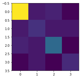
# plot sigma
plt.imshow(sigma, interpolation="nearest")
plt.show()
[4]:
q = 0.5  # set risk factor
budget = num_assets // 2  # set budget
penalty = num_assets  # set parameter to scale the budget penalty term

portfolio = PortfolioOptimization(
    expected_returns=mu, covariances=sigma, risk_factor=q, budget=budget
)
qp = portfolio.to_quadratic_program()
qp
[4]:
<QuadraticProgram: minimize 0.001270694296030004*x_0^2 + 7.340221669347328e-05..., 4 variables, 1 constraints, 'Portfolio optimization'>
ফলাফলগুলি সুন্দর বিন্যাসে মুদ্রণের জন্য আমরা কিছু উপযোগী কার্যপ্রণালী সংজ্ঞায়িত করি।
[5]:
def print_result(result):
    selection = result.x
    value = result.fval
    print("Optimal: selection {}, value {:.4f}".format(selection, value))

    eigenstate = result.min_eigen_solver_result.eigenstate
    probabilities = (
        eigenstate.binary_probabilities()
        if isinstance(eigenstate, QuasiDistribution)
        else {k: np.abs(v) ** 2 for k, v in eigenstate.to_dict().items()}
    )
    print("\n----------------- Full result ---------------------")
    print("selection\tvalue\t\tprobability")
    print("---------------------------------------------------")
    probabilities = sorted(probabilities.items(), key=lambda x: x[1], reverse=True)

    for k, v in probabilities:
        x = np.array([int(i) for i in list(reversed(k))])
        value = portfolio.to_quadratic_program().objective.evaluate(x)
        print("%10s\t%.4f\t\t%.4f" % (x, value, v))
NumPyMinimumEigensolver (একটি ধ্রুপদী তথ্যসূত্র (রেফারেন্স) হিসাবে)#
Lets solve the problem. First classically…
We can now use the Operator we built above without regard to the specifics of how it was created. We set the algorithm for the NumPyMinimumEigensolver so we can have a classical reference. The problem is set for 'ising'. Backend is not required since this is computed classically not using quantum computation. The result is returned as a dictionary.
[6]:
exact_mes = NumPyMinimumEigensolver()
exact_eigensolver = MinimumEigenOptimizer(exact_mes)

result = exact_eigensolver.solve(qp)

print_result(result)
Optimal: selection [1. 0. 0. 1.], value -0.0149

----------------- Full result ---------------------
selection       value           probability
---------------------------------------------------
 [1 0 0 1]      -0.0149         1.0000
Solution using SamplingVQE#
We can now use the Sampling Variational Quantum Eigensolver (SamplingVQE) to solve the problem. We will specify the optimizer and variational form to be used.
[7]:
from qiskit_algorithms.utils import algorithm_globals

algorithm_globals.random_seed = 1234

cobyla = COBYLA()
cobyla.set_options(maxiter=500)
ry = TwoLocal(num_assets, "ry", "cz", reps=3, entanglement="full")
svqe_mes = SamplingVQE(sampler=Sampler(), ansatz=ry, optimizer=cobyla)
svqe = MinimumEigenOptimizer(svqe_mes)
result = svqe.solve(qp)

print_result(result)
Optimal: selection [1. 0. 0. 1.], value -0.0149

----------------- Full result ---------------------
selection       value           probability
---------------------------------------------------
 [0 1 1 0]      0.0008          0.8525
 [1 0 0 1]      -0.0149         0.0410
 [0 0 1 1]      -0.0010         0.0312
 [0 0 0 1]      -0.0008         0.0215
 [1 0 1 1]      -0.0150         0.0195
 [1 0 0 0]      -0.0140         0.0088
 [0 1 1 1]      -0.0000         0.0078
 [0 1 0 1]      0.0002          0.0078
 [0 1 0 0]      0.0009          0.0059
 [1 0 1 0]      -0.0140         0.0020
 [1 1 0 1]      -0.0139         0.0010
 [0 0 0 0]      0.0000          0.0010
Solution using QAOA#
We also show here a result using the Quantum Approximate Optimization Algorithm (QAOA). This is another variational algorithm and it uses an internal variational form that is created based on the problem.
[8]:
algorithm_globals.random_seed = 1234

cobyla = COBYLA()
cobyla.set_options(maxiter=250)
qaoa_mes = QAOA(sampler=Sampler(), optimizer=cobyla, reps=3)
qaoa = MinimumEigenOptimizer(qaoa_mes)
result = qaoa.solve(qp)

print_result(result)
Optimal: selection [1. 0. 0. 1.], value -0.0149

----------------- Full result ---------------------
selection       value           probability
---------------------------------------------------
 [1 0 0 1]      -0.0149         0.1797
 [1 0 1 0]      -0.0140         0.1729
 [1 1 0 0]      -0.0130         0.1641
 [0 0 1 1]      -0.0010         0.1592
 [0 1 1 0]      0.0008          0.1553
 [0 1 0 1]      0.0002          0.1445
 [0 1 0 0]      0.0009          0.0049
 [1 1 0 1]      -0.0139         0.0039
 [1 1 1 1]      -0.0139         0.0039
 [0 0 0 0]      0.0000          0.0029
 [1 0 0 0]      -0.0140         0.0029
 [0 0 1 0]      -0.0001         0.0020
 [0 1 1 1]      -0.0000         0.0010
 [1 1 1 0]      -0.0130         0.0010
 [0 0 0 1]      -0.0008         0.0010
 [1 0 1 1]      -0.0150         0.0010
[9]:
import qiskit.tools.jupyter

%qiskit_version_table
%qiskit_copyright
Version Information
| Software | Version |
|---|---|
qiskit | 0.45.0.dev0+ea871e0 |
qiskit_optimization | 0.6.0 |
qiskit_finance | 0.4.0 |
qiskit_aer | 0.12.2 |
qiskit_ibm_provider | 0.7.0 |
qiskit_algorithms | 0.3.0 |
| System information | |
| Python version | 3.9.7 |
| Python compiler | GCC 7.5.0 |
| Python build | default, Sep 16 2021 13:09:58 |
| OS | Linux |
| CPUs | 2 |
| Memory (Gb) | 5.7784271240234375 |
| Tue Sep 05 15:03:52 2023 EDT | |
This code is a part of Qiskit
© Copyright IBM 2017, 2023.
This code is licensed under the Apache License, Version 2.0. You may
obtain a copy of this license in the LICENSE.txt file in the root directory
of this source tree or at http://www.apache.org/licenses/LICENSE-2.0.
Any modifications or derivative works of this code must retain this
copyright notice, and modified files need to carry a notice indicating
that they have been altered from the originals.
[ ]: