নোট

এই পৃষ্ঠাটি docs/tutorials/05_bull_spread_pricing.ipynb থেকে নেয়া হয়েছে।

বুল স্প্রেডের মূল্য নির্ধারণ

ভূমিকা

ধরুন একটি bull spread স্ট্রাইক প্রাইস সহ \(K_1 < K_2\) এবং একটি অন্তর্নিহিত সম্পদ যার পরিপক্কতার স্পট মূল্য \(S_T\) একটি প্রদত্ত এলোমেলো বন্টন অনুসরণ করে। সংশ্লিষ্ট পরিশোধ ফাংশনটি সংজ্ঞায়িত করা হয়েছে:

\[\min\{\max\{S_T - K_1, 0\}, K_2 - K_1\}\]

নিম্নে বিস্তার অনুমানের উপর ভিত্তি করে একটি কোয়ান্টাম অ্যালগরিদম ব্যবহার করা হয় প্রত্যাশিত পেঅফ, অর্থাৎ ছাড়ের আগে ন্যায্য মূল্য অনুমান করা হয়েছে:

\[\mathbb{E}\left[ \min\{\max\{S_T - K_1, 0\}, K_2 - K_1\} \right]\]

একই সাথে, সম্পর্কযুক্ত \(\Delta\) অর্থাৎ স্পট দামের সাপেক্ষে বিকল্প দামের অন্তরীকরণ এভাবে সংজ্ঞাযিত:

\[\Delta = \mathbb{P}\left[K_1 \leq S \leq K_2\right]\]

উদ্দেশ্য অন্বয়ের (অবজেক্টিভ ফাংশন) আনুমানিকতা এবং কোয়ান্টাম কম্পিউটারগুলিতে বিকল্প মূল্য নির্ধারণ এবং ঝুঁকি বিশ্লেষণের একটি সাধারণ ভূমিকা নিম্নলিখিত গবেষণাপত্রগুলোতে দেওয়া হয়েছে:

• Quantum Risk Analysis. Woerner, Egger. 2018.

• Option Pricing using Quantum Computers. Stamatopoulos et al. 2019.

import matplotlib.pyplot as plt

%matplotlib inline
import numpy as np

from qiskit_algorithms import IterativeAmplitudeEstimation, EstimationProblem
from qiskit.circuit.library import LinearAmplitudeFunction
from qiskit_aer.primitives import Sampler
from qiskit_finance.circuit.library import LogNormalDistribution

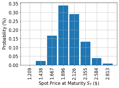
অনিশ্চয়তা মডেল

We construct a circuit to load a log-normal random distribution into a quantum state. The distribution is truncated to a given interval \([\text{low}, \text{high}]\) and discretized using \(2^n\) grid points, where \(n\) denotes the number of qubits used. The unitary operator corresponding to the circuit implements the following:

\[\big|0\rangle_{n} \mapsto \big|\psi\rangle_{n} = \sum_{i=0}^{2^n-1} \sqrt{p_i}\big|i\rangle_{n},\]

যেখানে math:p_i অগ্রভাগহীন এবং বিযুক্ত বিতরণগুলির সম্ভাবনা বোঝায় এবং \(i\) অ্যাফাইন ম্যাপ ব্যবহার করে ডান ব্যবধানে ম্যাপ করা হয়েছে:

\[\{0, \ldots, 2^n-1\} \ni i \mapsto \frac{\text{high} - \text{low}}{2^n - 1} * i + \text{low} \in [\text{low}, \text{high}]।.\]

# number of qubits to represent the uncertainty
num_uncertainty_qubits = 3

# parameters for considered random distribution
S = 2.0  # initial spot price
vol = 0.4  # volatility of 40%
r = 0.05  # annual interest rate of 4%
T = 40 / 365  # 40 days to maturity

# resulting parameters for log-normal distribution
mu = (r - 0.5 * vol**2) * T + np.log(S)
sigma = vol * np.sqrt(T)
mean = np.exp(mu + sigma**2 / 2)
variance = (np.exp(sigma**2) - 1) * np.exp(2 * mu + sigma**2)
stddev = np.sqrt(variance)

# lowest and highest value considered for the spot price; in between, an equidistant discretization is considered.
low = np.maximum(0, mean - 3 * stddev)
high = mean + 3 * stddev

# construct circuit for uncertainty model
uncertainty_model = LogNormalDistribution(
    num_uncertainty_qubits, mu=mu, sigma=sigma**2, bounds=(low, high)
)

# plot probability distribution
x = uncertainty_model.values
y = uncertainty_model.probabilities
plt.bar(x, y, width=0.2)
plt.xticks(x, size=15, rotation=90)
plt.yticks(size=15)
plt.grid()
plt.xlabel("Spot Price at Maturity $S_T$ (\$)", size=15)
plt.ylabel("Probability ($\%$)", size=15)
plt.show()

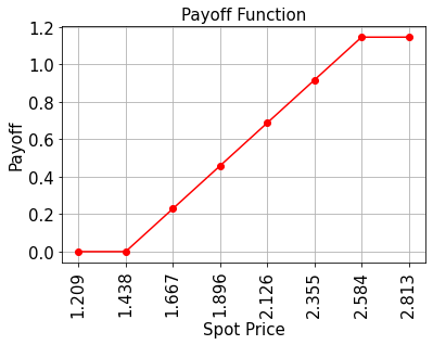
বেতনের ফাংশন

যখন স্পট মূল্য \(S_T\) পরিপক্ক অবস্থায় স্ট্রাইক মূল্য \(K_1\) এর চেয়ে কম তখন পে অফ অন্বয়ের মান শূন্য। তারপরে রৈখিকভাবে বৃদ্ধিপায় এবং এটি \(K_2\) দ্বারা আবদ্ধ। প্রয়োগটি দুইটি তুলনাকারী ব্যবহার করে, যা অ্যানসিলা কিউবিট ফ্লিপ করে \(\big|0\rangle\) থেকে \(\big|1\rangle\) তে যদি \(S_T \geq K_1\) এবং \(S_T \leq K_2\) হয়। এই অ্যানসিলাগুলো পেঅফ অন্বয়ের রৈখিক অংশ নিয়ন্ত্রণ করতে ব্যবহৃত হয়।

রৈখিক অংশ (linear part) টি অনুমান করতে এই পদ্ধতি ব্যবহার করা হয় - ছোট মান এর \(|y|\) এর জন্যে \(\sin^2(y + \pi/4) \approx y + 1/2\) হয়। সুতরাং, একটি প্রদত্ত আনুমানিক রিস্কেলিং ফ্যাক্টর \(c_\text{approx} \in [0, 1]\) এবং \(x \in [0, 1]\) এর জন্য আমরা বিবেচনা করি

\[\sin^2( \pi/2 * c_\text{approx} * ( x - 1/2 ) + \pi/4) \approx \pi/2 * c_\text{approx} * ( x - 1/2 ) + 1/2\]

ছোট :math:`c_{approx}`এর জন্যে।

আমরা খুব সহজেই একটি অপারেটর বানাতে পারি যেটা

\[\big|x\rangle \big|0\rangle \mapsto \big|x\rangle \left( \cos(a*x+b) \big|0\rangle + \sin(a*x+b) \big|1\rangle \right),\]

নিয়ন্ত্রিত Y-ঘূর্ণন ব্যবহার করে।

অবশেষে, আমরা শেষ কিউবিটে \(\big|1\rangle\) পরিমাপের সম্ভাবনাতে আগ্রহী, যেটা কিনা \(\sin^2(a*x+b)\) এর সাথে মিলে যাবার কথা। এই অনুমান গুলোর সাহায্যে আমরা আগ্রহের মানগুলির নিকটবর্তী মাত্রাগুলো পেয়ে যাব। যত ছোট \(c_{approx}\) এর মান হবে, তত ভালো হবে আমাদের প্রাপ্ত অনুমান। কিন্তু এখানে এটাও মাথায় রাখা দরকার যে যেহেতু অনুমানটি \(c_{approx}\) এর ওপরে নির্ভর তাই মূল্যায়নের কিউবিটগুলির সংখ্যা \(m\) সেই অনুসারে সামঞ্জস্য করা দরকার।

আনুমানিকতা সম্পর্কে আরো বিস্তারিত জানার জন্য, আমরা উল্লেখ করি: Quantum Risk Analysis. Woerner, Egger. 2018.

# set the strike price (should be within the low and the high value of the uncertainty)
strike_price_1 = 1.438
strike_price_2 = 2.584

# set the approximation scaling for the payoff function
rescaling_factor = 0.25

# setup piecewise linear objective fcuntion
breakpoints = [low, strike_price_1, strike_price_2]
slopes = [0, 1, 0]
offsets = [0, 0, strike_price_2 - strike_price_1]
f_min = 0
f_max = strike_price_2 - strike_price_1
bull_spread_objective = LinearAmplitudeFunction(
    num_uncertainty_qubits,
    slopes,
    offsets,
    domain=(low, high),
    image=(f_min, f_max),
    breakpoints=breakpoints,
    rescaling_factor=rescaling_factor,
)

# construct A operator for QAE for the payoff function by
# composing the uncertainty model and the objective
bull_spread = bull_spread_objective.compose(uncertainty_model, front=True)

# plot exact payoff function (evaluated on the grid of the uncertainty model)
x = uncertainty_model.values
y = np.minimum(np.maximum(0, x - strike_price_1), strike_price_2 - strike_price_1)
plt.plot(x, y, "ro-")
plt.grid()
plt.title("Payoff Function", size=15)
plt.xlabel("Spot Price", size=15)
plt.ylabel("Payoff", size=15)
plt.xticks(x, size=15, rotation=90)
plt.yticks(size=15)
plt.show()

# evaluate exact expected value (normalized to the [0, 1] interval)
exact_value = np.dot(uncertainty_model.probabilities, y)
exact_delta = sum(
    uncertainty_model.probabilities[np.logical_and(x >= strike_price_1, x <= strike_price_2)]
)
print("exact expected value:\t%.4f" % exact_value)
print("exact delta value:   \t%.4f" % exact_delta)

exact expected value:   0.5695
exact delta value:      0.9291

প্রত্যাশিত বেতন মূল্যনির্ধারণ

# set target precision and confidence level
epsilon = 0.01
alpha = 0.05

problem = EstimationProblem(
    state_preparation=bull_spread,
    objective_qubits=[num_uncertainty_qubits],
    post_processing=bull_spread_objective.post_processing,
)
# construct amplitude estimation
ae = IterativeAmplitudeEstimation(
    epsilon_target=epsilon, alpha=alpha, sampler=Sampler(run_options={"shots": 100, "seed": 75})
)

result = ae.estimate(problem)

conf_int = np.array(result.confidence_interval_processed)
print("Exact value:    \t%.4f" % exact_value)
print("Estimated value:\t%.4f" % result.estimation_processed)
print("Confidence interval: \t[%.4f, %.4f]" % tuple(conf_int))

Exact value:            0.5695
Estimated value:        0.5686
Confidence interval:    [0.5610, 0.5763]

ডেল্টা মূল্যায়ন

প্রত্যাশিত পে-অফের চেয়ে ডেল্টা মূল্যায়ন করা কিছুটা সহজ। একইভাবে প্রত্যাশিত বেতন হিসাবে, আমরা যেসবক্ষেত্রে \(K_1 \leq S_T \leq K_2\) হয়, সেগুলো শনাক্ত করতে একটি তুলনামূলক সার্কিট এবং একটি অ্যানসিলা কিউবিট ব্যবহার করি। তবে, যেহেতু আমরা কেবলমাত্র এই অবস্থার সত্য হওয়ার সম্ভাবনা সম্পর্কে আগ্রহী, তাই আমরা আর কোনো অনুমান ছাড়াই সরাসরি একটি অ্যানসিলা কিউবিটকে উদ্দেশ্যমূলক কিউবিট (অবজেক্টিভ কিউবিট) হিসাবে বিস্তার অনুমানে (অ্যামপ্লিটিউড এস্টিমেশন) ব্যবহার করতে পারি।

# setup piecewise linear objective fcuntion
breakpoints = [low, strike_price_1, strike_price_2]
slopes = [0, 0, 0]
offsets = [0, 1, 0]
f_min = 0
f_max = 1

bull_spread_delta_objective = LinearAmplitudeFunction(
    num_uncertainty_qubits,
    slopes,
    offsets,
    domain=(low, high),
    image=(f_min, f_max),
    breakpoints=breakpoints,
)  # no approximation necessary, hence no rescaling factor

# construct the A operator by stacking the uncertainty model and payoff function together
bull_spread_delta = bull_spread_delta_objective.compose(uncertainty_model, front=True)

# set target precision and confidence level
epsilon = 0.01
alpha = 0.05

problem = EstimationProblem(
    state_preparation=bull_spread_delta, objective_qubits=[num_uncertainty_qubits]
)
# construct amplitude estimation
ae_delta = IterativeAmplitudeEstimation(
    epsilon_target=epsilon, alpha=alpha, sampler=Sampler(run_options={"shots": 100, "seed": 75})
)

result_delta = ae_delta.estimate(problem)

conf_int = np.array(result_delta.confidence_interval)
print("Exact delta:    \t%.4f" % exact_delta)
print("Estimated value:\t%.4f" % result_delta.estimation)
print("Confidence interval: \t[%.4f, %.4f]" % tuple(conf_int))

Exact delta:            0.9291
Estimated value:        0.9290
Confidence interval:    [0.9269, 0.9312]

import qiskit.tools.jupyter

%qiskit_version_table
%qiskit_copyright

Version Information

Software	Version
qiskit	None
qiskit-terra	0.45.0.dev0+c626be7
qiskit_ibm_provider	0.6.1
qiskit_finance	0.4.0
qiskit_algorithms	0.2.0
qiskit_aer	0.12.0
System information
Python version	3.9.7
Python compiler	GCC 7.5.0
Python build	default, Sep 16 2021 13:09:58
OS	Linux
CPUs	2
Memory (Gb)	5.778430938720703
Fri Aug 18 16:15:46 2023 EDT

This code is a part of Qiskit

© Copyright IBM 2017, 2023.

This code is licensed under the Apache License, Version 2.0. You may
obtain a copy of this license in the LICENSE.txt file in the root directory
of this source tree or at http://www.apache.org/licenses/LICENSE-2.0.

Any modifications or derivative works of this code must retain this
copyright notice, and modified files need to carry a notice indicating
that they have been altered from the originals.