নোট
এই পৃষ্ঠাটি docs/tutorials/07_asian_barrier_spread_pricing.ipynb থেকে বানানো হয়েছে।
এশিয়ান ব্যারিয়ার স্প্রেডের মূল্য নির্ধারণ#
ভূমিকা#
একটি এশিয়ান বাধা বিস্তার 3 টি ভিন্ন ধরনের বিকল্পের সংমিশ্রণ, এবং যেমন, একাধিক সম্ভাব্য বৈশিষ্ট্যগুলিকে একত্রিত করে যা Qiskit ফাইন্যান্স বিকল্প মূল্য কাঠামো সমর্থন করে:
Asian option: পরিশোধিত সময়কাল বিবেচিত গড় দামের উপর নির্ভর করে।
Barrier Option: নির্ধারিত সময়সীমার মধ্যে যে কোনো সময় একটি নির্দিষ্ট সীমা অতিক্রম করলে পরিশোধ শূন্য।
(Bull) Spread: পরিশোধ শূন্য থেকে শুরু, রৈখিক বৃদ্ধি, ধ্রুবক থেকে শুরু করে একটি টুকরো রৈখিক ফাংশন অনুসরণ করে (গড় মূল্যের উপর নির্ভর করে)।
Suppose strike prices \(K_1 < K_2\) and time periods \(t=1,2\), with corresponding spot prices \((S_1, S_2)\) following a given multivariate distribution (e.g. generated by some stochastic process), and a barrier threshold \(B>0\). The corresponding payoff function is defined as
নিম্নে, একটি বিস্তার হিসাবের (অ্যামপ্লিটিউড) উপর নির্ভরশীল কোয়ান্টাম অ্যালগরিদম ব্যবহার করে প্রত্যাশিত পে-অফ, যা হলো ছাড় দেয়ার আগের আদর্শমূল্য, অনুমান করা হয়েছে
উদ্দেশ্য অন্বয়ের (অবজেক্টিভ ফাংশন) আনুমানিকতা এবং কোয়ান্টাম কম্পিউটারগুলিতে বিকল্প মূল্য নির্ধারণ এবং ঝুঁকি বিশ্লেষণের একটি সাধারণ ভূমিকা নিম্নলিখিত গবেষণাপত্রগুলোতে দেওয়া হয়েছে:
[1]:
import matplotlib.pyplot as plt
from scipy.interpolate import griddata

%matplotlib inline
import numpy as np

from qiskit import QuantumRegister, QuantumCircuit, AncillaRegister, transpile
from qiskit.circuit.library import IntegerComparator, WeightedAdder, LinearAmplitudeFunction
from qiskit_algorithms import IterativeAmplitudeEstimation, EstimationProblem
from qiskit_aer.primitives import Sampler
from qiskit_finance.circuit.library import LogNormalDistribution
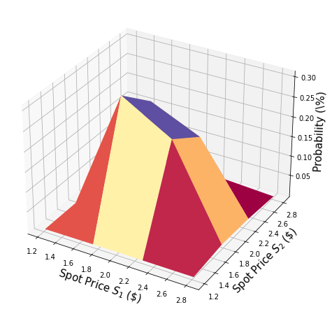
অনিশ্চয়তা মডেল#
We construct a circuit to load a multivariate log-normal random distribution into a quantum state on \(n\) qubits. For every dimension \(j = 1,\ldots,d\), the distribution is truncated to a given interval \([\text{low}_j, \text{high}_j]\) and discretized using \(2^{n_j}\) grid points, where \(n_j\) denotes the number of qubits used to represent dimension \(j\), i.e., \(n_1+\ldots+n_d = n\). The unitary operator corresponding to the circuit implements the following:
যেখানে math:p_{i_1ldots i_d} কাটা এবং বিযুক্ত বিতরণগুলির সম্ভাবনা বোঝায় এবং \(i_j\) অ্যাফাইন ম্যাপ ব্যবহার করে ডান ব্যবধানে ম্যাপ করা হয়েছে:
সরলতার জন্য, আমরা ধরি উভয় স্টক মূল্য স্বাধীন এবং অভিন্ন বিতরণ। এই অনুমানটি কেবল নিচের প্যারামেট্রাইজেশনকে সহজ করে এবং সহজেই আরও জটিল এবং correlated করা যেতে পারে বহুবিধ বিতরণকে। বর্তমান বাস্তবায়নের জন্য একমাত্র গুরুত্বপূর্ণ অনুমান হল যে বিভিন্ন মাত্রার বিচ্ছিন্নতা গ্রিডের একই ধাপের আকার রয়েছে।
[2]:
# number of qubits per dimension to represent the uncertainty
num_uncertainty_qubits = 2

# parameters for considered random distribution
S = 2.0  # initial spot price
vol = 0.4  # volatility of 40%
r = 0.05  # annual interest rate of 4%
T = 40 / 365  # 40 days to maturity

# resulting parameters for log-normal distribution
mu = (r - 0.5 * vol**2) * T + np.log(S)
sigma = vol * np.sqrt(T)
mean = np.exp(mu + sigma**2 / 2)
variance = (np.exp(sigma**2) - 1) * np.exp(2 * mu + sigma**2)
stddev = np.sqrt(variance)

# lowest and highest value considered for the spot price; in between, an equidistant discretization is considered.
low = np.maximum(0, mean - 3 * stddev)
high = mean + 3 * stddev

# map to higher dimensional distribution
# for simplicity assuming dimensions are independent and identically distributed)
dimension = 2
num_qubits = [num_uncertainty_qubits] * dimension
low = low * np.ones(dimension)
high = high * np.ones(dimension)
mu = mu * np.ones(dimension)
cov = sigma**2 * np.eye(dimension)

# construct circuit
u = LogNormalDistribution(num_qubits=num_qubits, mu=mu, sigma=cov, bounds=(list(zip(low, high))))
[3]:
# plot PDF of uncertainty model
x = [v[0] for v in u.values]
y = [v[1] for v in u.values]
z = u.probabilities
# z = map(float, z)
# z = list(map(float, z))
resolution = np.array([2**n for n in num_qubits]) * 1j
grid_x, grid_y = np.mgrid[min(x) : max(x) : resolution[0], min(y) : max(y) : resolution[1]]
grid_z = griddata((x, y), z, (grid_x, grid_y))
plt.figure(figsize=(10, 8))
ax = plt.axes(projection="3d")
ax.plot_surface(grid_x, grid_y, grid_z, cmap=plt.cm.Spectral)
ax.set_xlabel("Spot Price $S_1$ (\$)", size=15)
ax.set_ylabel("Spot Price $S_2$ (\$)", size=15)
ax.set_zlabel("Probability (\%)", size=15)
plt.show()
বেতনের অপেক্ষক#
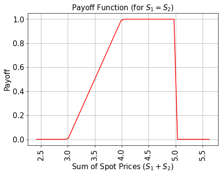
সরলতার জন্য, আমরা স্পট মূল্যের সমষ্টিকে তাদের গড়ের পরিবর্তে বিবেচনা করি। ফলাফলটি মাত্র ২ দ্বারা ভাগ করে গড়তে রূপান্তরিত করা যেতে পারে।
পে -অফ ফাংশন শূন্যের সমান হয় যতক্ষণ স্পট প্রাইসের যোগফল \((S_1 + S_2)\) স্ট্রাইক প্রাইস \(K_1\) এর চেয়ে কম হয় এবং তারপর রৈখিকভাবে বৃদ্ধি পায় যতক্ষণ না স্পট প্রাইসের যোগফল \(K_2\) এ পৌঁছায়। তারপরে পরিশোধ \(K_2 - K_1\)- তে স্থির থাকে যদি না দুটি স্পটের দাম বাধা থ্রেশহোল্ড \(B\) অতিক্রম করে, তাহলে পরিশোধ অবিলম্বে শূন্যে চলে যায়। বাস্তবায়ন প্রথমে একটি ওজনযুক্ত সমষ্টি অপারেটর ব্যবহার করে স্পট মূল্যের যোগফলকে একটি আনিসিলা রেজিস্টারে গণনা করে, এবং তারপর একটি তুলনাকারী ব্যবহার করে, যা একটি অ্যানসিলা কিউবিটকে \(\big|0\rangle\) থেকে \(\big|1\rangle\) if \((S_1 + S_2) \geq K_1\) এবং আরেকটি তুলনাকারী/আনসিলা কেস ধরার জন্য যে \((S_1 + S_2) \geq K_2\)। এই আনুষঙ্গিকগুলি পরিশোধ ফাংশনের রৈখিক অংশ নিয়ন্ত্রণ করতে ব্যবহৃত হয়।
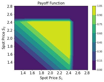
উপরন্তু, আমরা প্রতিটি সময় ধাপের জন্য আরেকটি আনসিলা ভেরিয়েবল যোগ করি এবং \(S_1\), যথাক্রমে \(S_2\), বাধা সীমা \(B\) অতিক্রম করে কিনা তা পরীক্ষা করার জন্য অতিরিক্ত তুলনাকারী ব্যবহার করি। পাওনা ফাংশন শুধুমাত্র তখনই প্রয়োগ করা হয় যদি \(S_1, S_2 \leq B\)।
রৈখিক অংশটি অনুমান করতে এই পদ্ধতি ব্যবহার করা হয়। আমরা ছোট \(|y|\) এর জন্য \(\sin^2(y + \pi/4) \approx y + 1/2\) ব্যবহার করি। সুতরাং, একটি প্রদত্ত আনুমানিক স্কেলিং ফ্যাক্টর \(c_\text{approx} \in [0, 1]\) এবং \(x \in [0, 1]\) এর জন্য আমরা বিবেচনা করি
for small \(c_\text{approx}\).
আমরা খুব সহজেই একটি অপারেটর বানাতে পারি যেটা
নিয়ন্ত্রিত Y-ঘূর্ণন ব্যবহার করে।
অবশেষে, আমরা শেষ কুইবিটে \(\big|1\rangle\) পরিমাপের সম্ভাবনাতে আগ্রহী, যেটা কিনা \(\sin^2(a*x+b)\) এর সাথে মিলে যাবার কথা। এই অনুমান গুলোর সাহায্যে আমরা আগ্রহের মানগুলির নিকটবর্তী মাত্রাগুলো পেয়ে যাব। যত ছোট \(c_{approx}\) এর মান হবে, তত আমাদের প্রাপ্ত অনুমান ভালো হবে। কিন্তু এখানে এটাও মাথায় রাখা দরকার যে যেহেতু অনুমানটি \(c_{approx}\) এর ওপরে নির্ভর তাই মূল্যায়নের কিউবিটগুলির সংখ্যা \(m\) সেই অনুসারে সামঞ্জস্য করা দরকার।
এই অনুমান বিষয়ে বিশদে জানার জন্যে: Quantum Risk Analysis. Woerner, Egger. 2018. দেখুন
যেহেতু ওজনযুক্ত সমষ্টি অপারেটর (তার বর্তমান বাস্তবায়নে) শুধুমাত্র পূর্ণসংখ্যার সমষ্টি করতে পারে, তাই ফলাফলটি অনুমান করার জন্য আমাদের মূল রেঞ্জ থেকে প্রতিনিধিত্বযোগ্য পরিসরে ম্যাপ করতে হবে এবং ফলাফলটি ব্যাখ্যা করার আগে এই ম্যাপিংটিকে বিপরীত করতে হবে। ম্যাপিং মূলত উপরের অনিশ্চয়তা মডেলের প্রেক্ষাপটে বর্ণিত অ্যাফাইন ম্যাপিংয়ের সাথে মিলে যায়।
[4]:
# determine number of qubits required to represent total loss
weights = []
for n in num_qubits:
    for i in range(n):
        weights += [2**i]

# create aggregation circuit
agg = WeightedAdder(sum(num_qubits), weights)
n_s = agg.num_sum_qubits
n_aux = agg.num_qubits - n_s - agg.num_state_qubits  # number of additional qubits
[5]:
# set the strike price (should be within the low and the high value of the uncertainty)
strike_price_1 = 3
strike_price_2 = 4

# set the barrier threshold
barrier = 2.5

# map strike prices and barrier threshold from [low, high] to {0, ..., 2^n-1}
max_value = 2**n_s - 1
low_ = low[0]
high_ = high[0]

mapped_strike_price_1 = (
    (strike_price_1 - dimension * low_) / (high_ - low_) * (2**num_uncertainty_qubits - 1)
)
mapped_strike_price_2 = (
    (strike_price_2 - dimension * low_) / (high_ - low_) * (2**num_uncertainty_qubits - 1)
)
mapped_barrier = (barrier - low) / (high - low) * (2**num_uncertainty_qubits - 1)
[6]:
# condition and condition result
conditions = []
barrier_thresholds = [2] * dimension
n_aux_conditions = 0
for i in range(dimension):
    # target dimension of random distribution and corresponding condition (which is required to be True)
    comparator = IntegerComparator(num_qubits[i], mapped_barrier[i] + 1, geq=False)
    n_aux_conditions = max(n_aux_conditions, comparator.num_ancillas)
    conditions += [comparator]
[7]:
# set the approximation scaling for the payoff function
c_approx = 0.25

# setup piecewise linear objective fcuntion
breakpoints = [0, mapped_strike_price_1, mapped_strike_price_2]
slopes = [0, 1, 0]
offsets = [0, 0, mapped_strike_price_2 - mapped_strike_price_1]
f_min = 0
f_max = mapped_strike_price_2 - mapped_strike_price_1
objective = LinearAmplitudeFunction(
    n_s,
    slopes,
    offsets,
    domain=(0, max_value),
    image=(f_min, f_max),
    rescaling_factor=c_approx,
    breakpoints=breakpoints,
)
[8]:
# define overall multivariate problem
qr_state = QuantumRegister(u.num_qubits, "state")  # to load the probability distribution
qr_obj = QuantumRegister(1, "obj")  # to encode the function values
ar_sum = AncillaRegister(n_s, "sum")  # number of qubits used to encode the sum
ar_cond = AncillaRegister(len(conditions) + 1, "conditions")
ar = AncillaRegister(
    max(n_aux, n_aux_conditions, objective.num_ancillas), "work"
)  # additional qubits

objective_index = u.num_qubits

# define the circuit
asian_barrier_spread = QuantumCircuit(qr_state, qr_obj, ar_cond, ar_sum, ar)

# load the probability distribution
asian_barrier_spread.append(u, qr_state)

# apply the conditions
for i, cond in enumerate(conditions):
    state_qubits = qr_state[(num_uncertainty_qubits * i) : (num_uncertainty_qubits * (i + 1))]
    asian_barrier_spread.append(cond, state_qubits + [ar_cond[i]] + ar[: cond.num_ancillas])

# aggregate the conditions on a single qubit
asian_barrier_spread.mcx(ar_cond[:-1], ar_cond[-1])

# apply the aggregation function controlled on the condition
asian_barrier_spread.append(agg.control(), [ar_cond[-1]] + qr_state[:] + ar_sum[:] + ar[:n_aux])

# apply the payoff function
asian_barrier_spread.append(objective, ar_sum[:] + qr_obj[:] + ar[: objective.num_ancillas])

# uncompute the aggregation
asian_barrier_spread.append(
    agg.inverse().control(), [ar_cond[-1]] + qr_state[:] + ar_sum[:] + ar[:n_aux]
)

# uncompute the conditions
asian_barrier_spread.mcx(ar_cond[:-1], ar_cond[-1])

for j, cond in enumerate(reversed(conditions)):
    i = len(conditions) - j - 1
    state_qubits = qr_state[(num_uncertainty_qubits * i) : (num_uncertainty_qubits * (i + 1))]
    asian_barrier_spread.append(
        cond.inverse(), state_qubits + [ar_cond[i]] + ar[: cond.num_ancillas]
    )

print(asian_barrier_spread.draw())
print("objective qubit index", objective_index)
              ┌───────┐┌──────┐             ┌───────────┐      ┌──────────────┐»
     state_0: ┤0      ├┤0     ├─────────────┤1          ├──────┤1             ├»
              │       ││      │             │           │      │              │»
     state_1: ┤1      ├┤1     ├─────────────┤2          ├──────┤2             ├»
              │  P(X) ││      │┌──────┐     │           │      │              │»
     state_2: ┤2      ├┤      ├┤0     ├─────┤3          ├──────┤3             ├»
              │       ││      ││      │     │           │      │              │»
     state_3: ┤3      ├┤      ├┤1     ├─────┤4          ├──────┤4             ├»
              └───────┘│      ││      │     │           │┌────┐│              │»
         obj: ─────────┤      ├┤      ├─────┤           ├┤3   ├┤              ├»
                       │      ││      │     │           ││    ││              │»
conditions_0: ─────────┤2     ├┤      ├──■──┤           ├┤    ├┤              ├»
                       │  cmp ││      │  │  │           ││    ││              │»
conditions_1: ─────────┤      ├┤2     ├──■──┤           ├┤    ├┤              ├»
                       │      ││  cmp │┌─┴─┐│   c_adder ││    ││   c_adder_dg │»
conditions_2: ─────────┤      ├┤      ├┤ X ├┤0          ├┤    ├┤0             ├»
                       │      ││      │└───┘│           ││    ││              │»
       sum_0: ─────────┤      ├┤      ├─────┤5          ├┤0   ├┤5             ├»
                       │      ││      │     │           ││  F ││              │»
       sum_1: ─────────┤      ├┤      ├─────┤6          ├┤1   ├┤6             ├»
                       │      ││      │     │           ││    ││              │»
       sum_2: ─────────┤      ├┤      ├─────┤7          ├┤2   ├┤7             ├»
                       │      ││      │     │           ││    ││              │»
      work_0: ─────────┤3     ├┤3     ├─────┤8          ├┤4   ├┤8             ├»
                       └──────┘└──────┘     │           ││    ││              │»
      work_1: ──────────────────────────────┤9          ├┤5   ├┤9             ├»
                                            │           ││    ││              │»
      work_2: ──────────────────────────────┤10         ├┤6   ├┤10            ├»
                                            └───────────┘└────┘└──────────────┘»
«                              ┌─────────┐
«     state_0: ────────────────┤0        ├
«                              │         │
«     state_1: ────────────────┤1        ├
«                   ┌─────────┐│         │
«     state_2: ─────┤0        ├┤         ├
«                   │         ││         │
«     state_3: ─────┤1        ├┤         ├
«                   │         ││         │
«         obj: ─────┤         ├┤         ├
«                   │         ││         │
«conditions_0: ──■──┤         ├┤2        ├
«                │  │         ││  cmp_dg │
«conditions_1: ──■──┤2        ├┤         ├
«              ┌─┴─┐│  cmp_dg ││         │
«conditions_2: ┤ X ├┤         ├┤         ├
«              └───┘│         ││         │
«       sum_0: ─────┤         ├┤         ├
«                   │         ││         │
«       sum_1: ─────┤         ├┤         ├
«                   │         ││         │
«       sum_2: ─────┤         ├┤         ├
«                   │         ││         │
«      work_0: ─────┤3        ├┤3        ├
«                   └─────────┘└─────────┘
«      work_1: ───────────────────────────
«
«      work_2: ───────────────────────────
«
objective qubit index 4
[9]:
# plot exact payoff function
plt.figure(figsize=(7, 5))
x = np.linspace(sum(low), sum(high))
y = (x <= 5) * np.minimum(np.maximum(0, x - strike_price_1), strike_price_2 - strike_price_1)
plt.plot(x, y, "r-")
plt.grid()
plt.title("Payoff Function (for $S_1 = S_2$)", size=15)
plt.xlabel("Sum of Spot Prices ($S_1 + S_2)$", size=15)
plt.ylabel("Payoff", size=15)
plt.xticks(size=15, rotation=90)
plt.yticks(size=15)
plt.show()
[10]:
# plot contour of payoff function with respect to both time steps, including barrier
plt.figure(figsize=(7, 5))
z = np.zeros((17, 17))
x = np.linspace(low[0], high[0], 17)
y = np.linspace(low[1], high[1], 17)
for i, x_ in enumerate(x):
    for j, y_ in enumerate(y):
        z[i, j] = np.minimum(
            np.maximum(0, x_ + y_ - strike_price_1), strike_price_2 - strike_price_1
        )
        if x_ > barrier or y_ > barrier:
            z[i, j] = 0

plt.title("Payoff Function", size=15)
plt.contourf(x, y, z)
plt.colorbar()
plt.xlabel("Spot Price $S_1$", size=15)
plt.ylabel("Spot Price $S_2$", size=15)
plt.xticks(size=15)
plt.yticks(size=15)
plt.show()
[11]:
# evaluate exact expected value
sum_values = np.sum(u.values, axis=1)
payoff = np.minimum(np.maximum(sum_values - strike_price_1, 0), strike_price_2 - strike_price_1)
leq_barrier = [np.max(v) <= barrier for v in u.values]
exact_value = np.dot(u.probabilities[leq_barrier], payoff[leq_barrier])
print("exact expected value:\t%.4f" % exact_value)
exact expected value: 0.8023
প্রত্যাশিত বেতন মূল্যনির্ধারণ কর#
আমরা প্রথমে কোয়ান্টাম সার্কিটটিকে সিমুলেট করে এবং উদ্দেশ্য কিউবিটে \(|1\rangle\) অবস্থা পরিমাপের ফলে সম্ভাব্যতা বিশ্লেষণ করে যাচাই করি।
[12]:
num_state_qubits = asian_barrier_spread.num_qubits - asian_barrier_spread.num_ancillas
print("state qubits: ", num_state_qubits)
transpiled = transpile(asian_barrier_spread, basis_gates=["u", "cx"])
print("circuit width:", transpiled.width())
print("circuit depth:", transpiled.depth())
state qubits:  5
circuit width: 14
circuit depth: 6373
[13]:
asian_barrier_spread_measure = asian_barrier_spread.measure_all(inplace=False)
sampler = Sampler()
job = sampler.run(asian_barrier_spread_measure)
[14]:
# evaluate the result
value = 0
probabilities = job.result().quasi_dists[0].binary_probabilities()
for i, prob in probabilities.items():
    if prob > 1e-4 and i[-num_state_qubits:][0] == "1":
        value += prob


# map value to original range
mapped_value = objective.post_processing(value) / (2**num_uncertainty_qubits - 1) * (high_ - low_)
print("Exact Operator Value:  %.4f" % value)
print("Mapped Operator value: %.4f" % mapped_value)
print("Exact Expected Payoff: %.4f" % exact_value)
Exact Operator Value:  0.6455
Mapped Operator value: 0.8705
Exact Expected Payoff: 0.8023
পরবর্তী আমরা প্রত্যাশিত পরিশোধ অনুমান করতে বিস্তার অনুমান ব্যবহার করি। মনে রাখবেন যে এটি কিছুটা সময় নিতে পারে কারণ আমরা প্রচুর সংখ্যক কিউবিটস অনুকরণ করছি। যেভাবে আমরা অপারেটরকে ডিজাইন করেছি (asian_barrier_spread) বোঝায় যে প্রকৃত অবস্থা কুইবিট সংখ্যা উল্লেখযোগ্যভাবে ছোট, এইভাবে, সামগ্রিক সিমুলেশন সময় কিছুটা কমাতে সাহায্য করে।
[15]:
# set target precision and confidence level
epsilon = 0.01
alpha = 0.05

problem = EstimationProblem(
    state_preparation=asian_barrier_spread,
    objective_qubits=[objective_index],
    post_processing=objective.post_processing,
)
# construct amplitude estimation
ae = IterativeAmplitudeEstimation(
    epsilon, alpha=alpha, sampler=Sampler(run_options={"shots": 100, "seed": 75})
)
[16]:
result = ae.estimate(problem)
[17]:
conf_int = (
    np.array(result.confidence_interval_processed)
    / (2**num_uncertainty_qubits - 1)
    * (high_ - low_)
)
print("Exact value:    \t%.4f" % exact_value)
print(
    "Estimated value:\t%.4f"
    % (result.estimation_processed / (2**num_uncertainty_qubits - 1) * (high_ - low_))
)
print("Confidence interval: \t[%.4f, %.4f]" % tuple(conf_int))
Exact value:            0.8023
Estimated value:        0.8320
Confidence interval:    [0.8264, 0.8376]
[18]:
import qiskit.tools.jupyter

%qiskit_version_table
%qiskit_copyright
Version Information
| Software | Version |
|---|---|
qiskit | None |
qiskit-terra | 0.45.0.dev0+c626be7 |
qiskit_aer | 0.12.0 |
qiskit_ibm_provider | 0.6.1 |
qiskit_algorithms | 0.2.0 |
qiskit_finance | 0.4.0 |
| System information | |
| Python version | 3.9.7 |
| Python compiler | GCC 7.5.0 |
| Python build | default, Sep 16 2021 13:09:58 |
| OS | Linux |
| CPUs | 2 |
| Memory (Gb) | 5.778430938720703 |
| Fri Aug 18 16:20:04 2023 EDT | |
This code is a part of Qiskit
© Copyright IBM 2017, 2023.
This code is licensed under the Apache License, Version 2.0. You may
obtain a copy of this license in the LICENSE.txt file in the root directory
of this source tree or at http://www.apache.org/licenses/LICENSE-2.0.
Any modifications or derivative works of this code must retain this
copyright notice, and modified files need to carry a notice indicating
that they have been altered from the originals.
[ ]: