নোট
এই পৃষ্ঠাটি docs/tutorials/00_amplitude_estimation.ipynb থেকে বানানো হয়েছে।
কোয়ান্টাম বিস্তার অনুমান#
প্রদত্ত \(\mathcal{A}\) অপারেটরটি যেভাবে কাজ করে,
কোয়ান্টাম বিস্তার অনুমান (QAE) হল \(|\Psi_1\rangle\) অবস্থার \(a\) বিস্তারের জন্য একটি অনুমান খুঁজে বের করার কাজ:
This task has first been investigated by Brassard et al. [1] in 2000 and their algorithm uses a combination of the Grover operator
where \(\mathcal{S}_0\) and \(\mathcal{S}_{\Psi_1}\) are reflections about the \(|0\rangle\) and \(|\Psi_1\rangle\) states, respectively, and phase estimation. However this algorithm, called AmplitudeEstimation in Qiskit Algorithms, requires large circuits and is computationally expensive. Therefore, other variants of QAE have been proposed, which we will showcase in this tutorial for a simple example.
আমাদের উদাহরণে, \(\mathcal{A}\) একটি বার্নোলি (Bernoulli) দৈব চল রাশি বর্ণনা করে (অজানা বলে ধরে নেওয়া হয়) সাফল্যের সম্ভাবনা \(p\):
একটি কোয়ান্টাম কম্পিউটারে আমরা এই অপারেটরকে একটি একক কিউবিটের \(Y\) অক্ষের চারদিকে ঘুরিয়ে মডেল করতে পারি
এই ক্ষেত্রে গ্রোভার অপারেটর বেশ সহজ
যার ক্ষমতা গণনা করা খুব সহজ: \(\mathcal{Q}^k = R_Y(2k\theta_p)\)।
We’ll fix the probability we want to estimate to \(p = 0.2\).
[1]:
p = 0.2
এখন আমরা \(\mathcal{A}\) এবং \(\mathcal{Q}\) এর জন্য বর্তনী (সার্কিট) সংজ্ঞায়িত করতে পারি।
[2]:
import numpy as np
from qiskit.circuit import QuantumCircuit


class BernoulliA(QuantumCircuit):
    """A circuit representing the Bernoulli A operator."""

    def __init__(self, probability):
        super().__init__(1)  # circuit on 1 qubit

        theta_p = 2 * np.arcsin(np.sqrt(probability))
        self.ry(theta_p, 0)


class BernoulliQ(QuantumCircuit):
    """A circuit representing the Bernoulli Q operator."""

    def __init__(self, probability):
        super().__init__(1)  # circuit on 1 qubit

        self._theta_p = 2 * np.arcsin(np.sqrt(probability))
        self.ry(2 * self._theta_p, 0)

    def power(self, k):
        # implement the efficient power of Q
        q_k = QuantumCircuit(1)
        q_k.ry(2 * k * self._theta_p, 0)
        return q_k
[3]:
A = BernoulliA(p)
Q = BernoulliQ(p)
Amplitude Estimation workflow#
Qiskit Algorithms implements several QAE algorithms that all derive from the AmplitudeEstimator interface. In the initializer we specify algorithm specific settings and the estimate method, which does all the work, takes an EstimationProblem as input and returns an
AmplitudeEstimationResult object. Since all QAE variants follow the same interface, we can use them all to solve the same problem instance.
Next, we’ll run all different QAE algorithms. To do so, we first define the estimation problem which will contain the \(\mathcal{A}\) and \(\mathcal{Q}\) operators as well as how to identify the \(|\Psi_1\rangle\) state, which in this simple example is just \(|1\rangle\).
[4]:
from qiskit_algorithms import EstimationProblem

problem = EstimationProblem(
    state_preparation=A,  # A operator
    grover_operator=Q,  # Q operator
    objective_qubits=[0],  # the "good" state Psi1 is identified as measuring |1> in qubit 0
)
To execute circuits we’ll use Sampler.
[5]:
from qiskit.primitives import Sampler

sampler = Sampler()
ক্যানোনিকাল এ.ই (Canonical AE)#
Now let’s solve this with the original QAE implementation by Brassard et al. [1].
[6]:
from qiskit_algorithms import AmplitudeEstimation

ae = AmplitudeEstimation(
    num_eval_qubits=3,  # the number of evaluation qubits specifies circuit width and accuracy
    sampler=sampler,
)
অ্যালগরিদম সংজ্ঞায়িত করার সাথে, আমরা estimate পদ্ধতিটি কল করতে পারি এবং এই সমস্যার সমাধান করতে পারি।
[7]:
ae_result = ae.estimate(problem)
অনুমানটি estimate key তে পাওয়া যায়:
[8]:
print(ae_result.estimation)
0.1464466
We see that this is not a very good estimate for our target of \(p=0.2\)! That’s due to the fact the canonical AE is restricted to a discrete grid, specified by the number of evaluation qubits:
[9]:
import matplotlib.pyplot as plt

# plot estimated values
gridpoints = list(ae_result.samples.keys())
probabilities = list(ae_result.samples.values())

plt.bar(gridpoints, probabilities, width=0.5 / len(probabilities))
plt.axvline(p, color="r", ls="--")
plt.xticks(size=15)
plt.yticks([0, 0.25, 0.5, 0.75, 1], size=15)
plt.title("Estimated Values", size=15)
plt.ylabel("Probability", size=15)
plt.xlabel(r"Amplitude $a$", size=15)
plt.ylim((0, 1))
plt.grid()
plt.show()
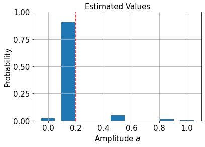
অনুমানের উন্নতির জন্য আমরা পরিমাপের সম্ভাব্যতাকে বিভক্ত করতে পারি এবং এই সম্ভাব্যতা বণ্টন তৈরির সর্বোচ্চ সম্ভাব্যতা নির্ণয়কারীকে হিসাব করতে পারি:
[10]:
print("Interpolated MLE estimator:", ae_result.mle)
Interpolated MLE estimator: 0.19999999406856905
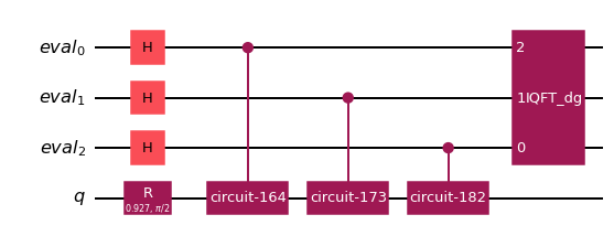
আমরা AE যে সার্কিটটি চালায় তার দিকে নজর দিতে পারি:
[11]:
ae_circuit = ae.construct_circuit(problem)
ae_circuit.decompose().draw(
    "mpl", style="iqx"
)  # decompose 1 level: exposes the Phase estimation circuit!
[11]:
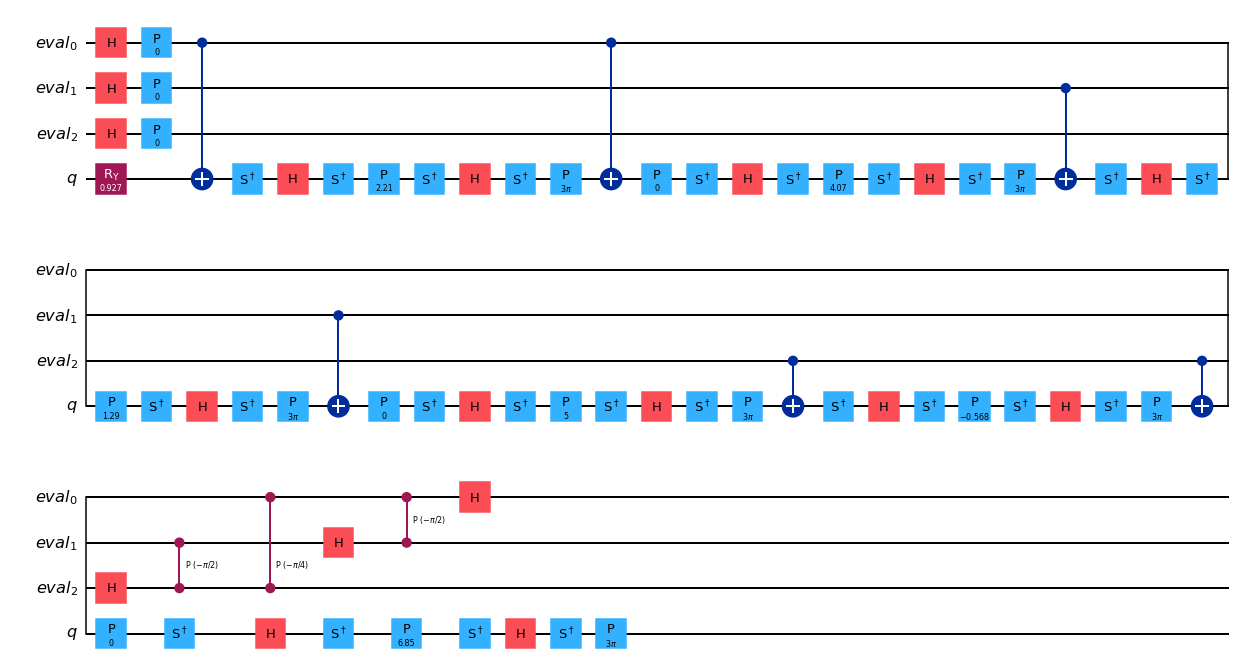
[12]:
from qiskit import transpile


basis_gates = ["h", "ry", "cry", "cx", "ccx", "p", "cp", "x", "s", "sdg", "y", "t", "cz"]
transpile(ae_circuit, basis_gates=basis_gates, optimization_level=2).draw("mpl", style="iqx")
[12]:
পুনরাবৃত্ত বিস্তার নির্ণয়#
[২] দেখুন।
[13]:
from qiskit_algorithms import IterativeAmplitudeEstimation

iae = IterativeAmplitudeEstimation(
    epsilon_target=0.01,  # target accuracy
    alpha=0.05,  # width of the confidence interval
    sampler=sampler,
)
iae_result = iae.estimate(problem)

print("Estimate:", iae_result.estimation)
Estimate: 0.2
এখানে সার্কিট শুধুমাত্র গ্রোভার পাওয়ার নিয়ে গঠিত এবং অনেক সস্তা!
[14]:
iae_circuit = iae.construct_circuit(problem, k=3)
iae_circuit.draw("mpl", style="iqx")
[14]:

সর্বাধিক সম্ভাব্যতা বিস্তার নির্ণয়#
[৩] দেখুন।
[15]:
from qiskit_algorithms import MaximumLikelihoodAmplitudeEstimation

mlae = MaximumLikelihoodAmplitudeEstimation(
    evaluation_schedule=3,  # log2 of the maximal Grover power
    sampler=sampler,
)
mlae_result = mlae.estimate(problem)

print("Estimate:", mlae_result.estimation)
Estimate: 0.20002237175368104
দ্রুততর বিস্তার নির্ণয়#
[৪] দেখুন।
[18]:
from qiskit_algorithms import FasterAmplitudeEstimation

fae = FasterAmplitudeEstimation(
    delta=0.01,  # target accuracy
    maxiter=3,  # determines the maximal power of the Grover operator
    sampler=sampler,
)
fae_result = fae.estimate(problem)

print("Estimate:", fae_result.estimation)
Estimate: 0.2030235918323876
তথ্যসূত্র (রেফারেন্স)#
[১] Quantum Amplitude Amplification and Estimation. Brassard et al (2000). https://arxiv.org/abs/quant-ph/0005055
[২] Iterative Quantum Amplitude Estimation. Grinko, D., Gacon, J., Zoufal, C., & Woerner, S. (2019). https://arxiv.org/abs/1912.05559
[৩] Amplitude Estimation without Phase Estimation. Suzuki, Y., Uno, S., Raymond, R., Tanaka, T., Onodera, T., & Yamamoto, N. (2019). https://arxiv.org/abs/1904.10246
[৪] Faster Amplitude Estimation. K. Nakaji (2020). https://arxiv.org/pdf/2003.02417.pdf
[17]:
import qiskit.tools.jupyter

%qiskit_version_table
%qiskit_copyright
Version Information
| Software | Version |
|---|---|
qiskit | None |
qiskit-terra | 0.45.0.dev0+c626be7 |
qiskit_ibm_provider | 0.6.1 |
qiskit_algorithms | 0.2.0 |
| System information | |
| Python version | 3.9.7 |
| Python compiler | GCC 7.5.0 |
| Python build | default, Sep 16 2021 13:09:58 |
| OS | Linux |
| CPUs | 2 |
| Memory (Gb) | 5.778430938720703 |
| Fri Aug 18 15:44:17 2023 EDT | |
This code is a part of Qiskit
© Copyright IBM 2017, 2023.
This code is licensed under the Apache License, Version 2.0. You may
obtain a copy of this license in the LICENSE.txt file in the root directory
of this source tree or at http://www.apache.org/licenses/LICENSE-2.0.
Any modifications or derivative works of this code must retain this
copyright notice, and modified files need to carry a notice indicating
that they have been altered from the originals.
[ ]: