নোট
এই পেজটি docs/tutorials/09_credit_risk_analysis.ipynb থেকে তৈরি হয়েছে।
ক্রেডিট ঝুঁকি বিশ্লেষণ#
ভূমিকা#
এই টিউটোরিয়াল দেখায় কিভাবে ক্রেডিট ঝুঁকি বিশ্লেষণের জন্য কোয়ান্টাম অ্যালগরিদম ব্যবহার করা যায়। আরো স্পষ্টভাবে, কিভাবে কোয়ান্টাম প্রশস্ততা অনুমান (QAE) প্রথাগত (ক্লাসিক্যাল) মন্টে কার্লো সিমুলেশন উপর একটি দ্বিঘাত গতি বৃদ্ধির সঙ্গে ঝুঁকি পরিমাপ অনুমান করতে ব্যবহার করা যেতে পারে। টিউটোরিয়ালটি নিম্নলিখিত গবেষণার উপর ভিত্তি করে:
Quantum Risk Analysis. Stefan Woerner, Daniel J. Egger. [Woerner2019]
Credit Risk Analysis using Quantum Computers. Egger et al. (2019) [Egger2019]
QAE- এর একটি সাধারণ ভূমিকা নিম্নলিখিত গবেষণায় পাওয়া যাবে:
টিউটোরিয়ালের গঠন নিম্নরূপ:
Problem Definition
Uncertainty Model
Expected Loss
Cumulative Distribution Function
Value at Risk
Conditional Value at Risk
[1]:
import numpy as np
import matplotlib.pyplot as plt

from qiskit import QuantumRegister, QuantumCircuit
from qiskit.circuit.library import IntegerComparator
from qiskit_algorithms import IterativeAmplitudeEstimation, EstimationProblem
from qiskit_aer.primitives import Sampler
সমস্যার সংজ্ঞায়ণ#
এই টিউটোরিয়ালে আমরা \(K\) সম্পদের একটি পোর্টফলিও এর ঋণের ঝুঁকি বিশ্লেষণ করতে চাই। প্রতিটি \(k\) সম্পদের ডিফল্ট বা পূর্বনির্ধারিত সম্ভাবনা একটি Gaussian Conditional Independence মডেল অনুসরণ করে, অর্থাৎ, একটি প্রদত্ত মান \(z\) যা স্ট্যান্ডার্ড normal বণ্টন কে অনুসরণকারী একটি সুপ্ত র্যান্ডম (দৈবচয়নের মাধ্যমে নির্বাচিত) চল রাশি \(Z\) থেকে স্যাম্পলিং করা হলে , \(k\) সম্পদ বা এ্যাসেটের ডিফল্ট সম্ভাবনা হবে
যেখানে \(F\) হল \(Z\) এর ক্রমবর্ধমান বন্টন ফাংশনকে বোঝায়, \(p_k^0\) হল \(z=0\) এর জন্য সম্পদ \(k\) এর ডিফল্ট সম্ভাব্যতা এবং \(\rho_k\) হল \(Z\) এর সাপেক্ষে সম্পদ \(k\) এর ডিফল্ট সম্ভাব্যতার সংবেদনশীলতা। এইভাবে, \(Z\) এর একটি সুনির্দিষ্ট উপলব্ধি দেওয়া হলে পৃথক ডিফল্ট ঘটনাগুলি একে অপরের থেকে স্বাধীন বলে ধরে নেওয়া হয়।
আমরা মোট লোকসানের ঝুঁকিপূর্ণতা বিশ্লেষণ করতে আগ্রহী
যেখানে \(\lambda_k\) সম্পদ \(k\) এর ডিফল্ট প্রদত্ত ক্ষতি বোঝায়, এবং \(Z\) দেওয়া আছে, \(X_k(Z)\) একটি বার্নোলি চল রাশিকে বোঝায় যা সম্পদ \(k\) এর ডিফল্ট ইভেন্টের প্রতিনিধিত্ব করে। আরো স্পষ্টভাবে, আমরা গড় মান \(\mathbb{E}[L]\), \(L\) এর ঝুঁকিতে (VaR) মান এবং \(L\) এর ঝুঁকিতে শর্তাধীন মান (যা প্রত্যাশিত শর্টফালও বলা হয়) সম্পর্কে আগ্রহী। যেখানে VaR এবং CVaR কে সংজ্ঞায়িত করা হয়েছে
যার confidence level \(\alpha \in [0, 1]\), এবং
বিবেচিত মডেল সম্পর্কে আরো বিস্তারিত জানার জন্য, দেখুন, যেমন, Regulatory Capital Modeling for Credit Risk. Marek Rutkowski, Silvio Tarca
The problem is defined by the following parameters:
number of qubits used to represent \(Z\), denoted by \(n_z\)
truncation value for \(Z\), denoted by \(z_{\text{max}}\), i.e., Z is assumed to take \(2^{n_z}\) equidistant values in \(\{-z_{max}, ..., +z_{max}\}\)
the base default probabilities for each asset \(p_0^k \in (0, 1)\), \(k=1, ..., K\)
sensitivities of the default probabilities with respect to \(Z\), denoted by \(\rho_k \in [0, 1)\)
loss given default for asset \(k\), denoted by \(\lambda_k\)
confidence level for VaR / CVaR \(\alpha \in [0, 1]\).
[2]:
# set problem parameters
n_z = 2
z_max = 2
z_values = np.linspace(-z_max, z_max, 2**n_z)
p_zeros = [0.15, 0.25]
rhos = [0.1, 0.05]
lgd = [1, 2]
K = len(p_zeros)
alpha = 0.05
অনিশ্চয়তা মডেল#
আমরা এখন একটি সার্কিট তৈরি করি যা অনিশ্চয়তা মডেল লোড করে। \(n_z\) qubits এর একটি রেজিস্টারে একটি কোয়ান্টাম অবস্থা তৈরি করে এটি অর্জন করা যায় যা একটি আদর্শ স্বাভাবিক বন্টন অনুসরণ করে \(Z\) কে প্রতিনিধিত্ব করে। এই অবস্থাটি তখন \(K\) qubits এর একটি দ্বিতীয় qubit রেজিস্টারে একক qubit Y- ঘূর্ণন নিয়ন্ত্রণ করতে ব্যবহৃত হয়, যেখানে \(k\) qubit এর \(|1\rangle\) অবস্থাটি asset \(k\) এর ডিফল্ট ঘটনাকে উপস্থাপন করে। ফলে কোয়ান্টাম অবস্থা হিসাবে লেখা যেতে পারে
যেখানে আমরা \(z_i\) দ্বারা \(i\)-তম মানটি বিচ্ছিন্ন এবং ছেঁটে দেওয়া \(Z\) [Egger2019] দ্বারা নির্দেশ করি।
[3]:
from qiskit_finance.circuit.library import GaussianConditionalIndependenceModel as GCI

u = GCI(n_z, z_max, p_zeros, rhos)
[4]:
u.draw()
[4]:
     ┌───────┐
q_0: ┤0      ├
     │       │
q_1: ┤1      ├
     │  P(X) │
q_2: ┤2      ├
     │       │
q_3: ┤3      ├
     └───────┘
We now use the simulator to validate the circuit that constructs \(|\Psi\rangle\) and compute the corresponding exact values for
expected loss \(\mathbb{E}[L]\)
PDF and CDF of \(L\)
value at risk \(VaR(L)\) and corresponding probability
conditional value at risk \(CVaR(L)\)
[5]:
u_measure = u.measure_all(inplace=False)
sampler = Sampler()
job = sampler.run(u_measure)
binary_probabilities = job.result().quasi_dists[0].binary_probabilities()
[6]:
# analyze uncertainty circuit and determine exact solutions
p_z = np.zeros(2**n_z)
p_default = np.zeros(K)
values = []
probabilities = []
num_qubits = u.num_qubits

for i, prob in binary_probabilities.items():
    # extract value of Z and corresponding probability
    i_normal = int(i[-n_z:], 2)
    p_z[i_normal] += prob

    # determine overall default probability for k
    loss = 0
    for k in range(K):
        if i[K - k - 1] == "1":
            p_default[k] += prob
            loss += lgd[k]

    values += [loss]
    probabilities += [prob]


values = np.array(values)
probabilities = np.array(probabilities)

expected_loss = np.dot(values, probabilities)
losses = np.sort(np.unique(values))
pdf = np.zeros(len(losses))
for i, v in enumerate(losses):
    pdf[i] += sum(probabilities[values == v])
cdf = np.cumsum(pdf)

i_var = np.argmax(cdf >= 1 - alpha)
exact_var = losses[i_var]
exact_cvar = np.dot(pdf[(i_var + 1) :], losses[(i_var + 1) :]) / sum(pdf[(i_var + 1) :])
[7]:
print("Expected Loss E[L]:                %.4f" % expected_loss)
print("Value at Risk VaR[L]:              %.4f" % exact_var)
print("P[L <= VaR[L]]:                    %.4f" % cdf[exact_var])
print("Conditional Value at Risk CVaR[L]: %.4f" % exact_cvar)
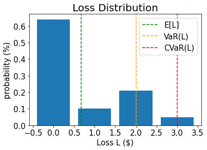
Expected Loss E[L]:                0.6641
Value at Risk VaR[L]:              2.0000
P[L <= VaR[L]]:                    0.9521
Conditional Value at Risk CVaR[L]: 3.0000
[8]:
# plot loss PDF, expected loss, var, and cvar
plt.bar(losses, pdf)
plt.axvline(expected_loss, color="green", linestyle="--", label="E[L]")
plt.axvline(exact_var, color="orange", linestyle="--", label="VaR(L)")
plt.axvline(exact_cvar, color="red", linestyle="--", label="CVaR(L)")
plt.legend(fontsize=15)
plt.xlabel("Loss L ($)", size=15)
plt.ylabel("probability (%)", size=15)
plt.title("Loss Distribution", size=20)
plt.xticks(size=15)
plt.yticks(size=15)
plt.show()
[9]:
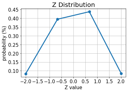
# plot results for Z
plt.plot(z_values, p_z, "o-", linewidth=3, markersize=8)
plt.grid()
plt.xlabel("Z value", size=15)
plt.ylabel("probability (%)", size=15)
plt.title("Z Distribution", size=20)
plt.xticks(size=15)
plt.yticks(size=15)
plt.show()
[10]:
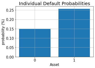
# plot results for default probabilities
plt.bar(range(K), p_default)
plt.xlabel("Asset", size=15)
plt.ylabel("probability (%)", size=15)
plt.title("Individual Default Probabilities", size=20)
plt.xticks(range(K), size=15)
plt.yticks(size=15)
plt.grid()
plt.show()
গড় লোকসান#
গড় লোকসান অনুমান করতে, আমরা প্রথমে ওজনযুক্ত সমষ্টি অপারেটরটি প্রয়োগ করে পৃথক লোকসান সমষ্টি করি।
ফলাফল বর্ণনা করার জন্য প্রয়োজনীয় কিউবিটগুলো হল
একবার আমাদের একটি কোয়ান্টাম রেজিস্টারে মোট ক্ষতি বন্টন হয়ে গেলে, আমরা [Woerner2019] এ বর্ণিত কৌশলগুলি ব্যবহার করে মোট ক্ষতির চিত্রায়ন তৈরি করতে পারি \(L \in \{0, ..., 2^{n_s}-1\}\) একটি অপারেটর দ্বারা একটি অব্জেক্টিভ কিউবিট এর বিস্তার
যা গড় লোকসান মূল্যায়ন করতে বিস্তার অনুমান চালাতে দেয়।
[11]:
# add Z qubits with weight/loss 0
from qiskit.circuit.library import WeightedAdder

agg = WeightedAdder(n_z + K, [0] * n_z + lgd)
[12]:
from qiskit.circuit.library import LinearAmplitudeFunction

# define linear objective function
breakpoints = [0]
slopes = [1]
offsets = [0]
f_min = 0
f_max = sum(lgd)
c_approx = 0.25

objective = LinearAmplitudeFunction(
    agg.num_sum_qubits,
    slope=slopes,
    offset=offsets,
    # max value that can be reached by the qubit register (will not always be reached)
    domain=(0, 2**agg.num_sum_qubits - 1),
    image=(f_min, f_max),
    rescaling_factor=c_approx,
    breakpoints=breakpoints,
)
মান বা অবস্থা প্রস্তুতিকরন বর্তনী তৈরি কর:
[13]:
# define the registers for convenience and readability
qr_state = QuantumRegister(u.num_qubits, "state")
qr_sum = QuantumRegister(agg.num_sum_qubits, "sum")
qr_carry = QuantumRegister(agg.num_carry_qubits, "carry")
qr_obj = QuantumRegister(1, "objective")

# define the circuit
state_preparation = QuantumCircuit(qr_state, qr_obj, qr_sum, qr_carry, name="A")

# load the random variable
state_preparation.append(u.to_gate(), qr_state)

# aggregate
state_preparation.append(agg.to_gate(), qr_state[:] + qr_sum[:] + qr_carry[:])

# linear objective function
state_preparation.append(objective.to_gate(), qr_sum[:] + qr_obj[:])

# uncompute aggregation
state_preparation.append(agg.to_gate().inverse(), qr_state[:] + qr_sum[:] + qr_carry[:])

# draw the circuit
state_preparation.draw()
[13]:
           ┌───────┐┌────────┐      ┌───────────┐
  state_0: ┤0      ├┤0       ├──────┤0          ├
           │       ││        │      │           │
  state_1: ┤1      ├┤1       ├──────┤1          ├
           │  P(X) ││        │      │           │
  state_2: ┤2      ├┤2       ├──────┤2          ├
           │       ││        │      │           │
  state_3: ┤3      ├┤3       ├──────┤3          ├
           └───────┘│  adder │┌────┐│  adder_dg │
objective: ─────────┤        ├┤2   ├┤           ├
                    │        ││    ││           │
    sum_0: ─────────┤4       ├┤0 F ├┤4          ├
                    │        ││    ││           │
    sum_1: ─────────┤5       ├┤1   ├┤5          ├
                    │        │└────┘│           │
    carry: ─────────┤6       ├──────┤6          ├
                    └────────┘      └───────────┘
আমরা গড় ক্ষতির অনুমান করার জন্য QAE ব্যবহার করার আগে, আমরা কোয়ান্টাম সার্কিটকে অব্জেক্টিভ ফাংশনকে প্রতিনিধিত্ব করে কেবলমাত্র এটিকে সরাসরি অনুকরণ করে এবং \(|1\rangle\) অবস্থায় থাকা অব্জেক্টিভ qubit এর সম্ভাব্যতা বিশ্লেষণ করে, অর্থাৎ QAE শেষ পর্যন্ত আনুমানিক হবে।
[14]:
state_preparation_measure = state_preparation.measure_all(inplace=False)
sampler = Sampler()
job = sampler.run(state_preparation_measure)
binary_probabilities = job.result().quasi_dists[0].binary_probabilities()
[15]:
# evaluate the result
value = 0
for i, prob in binary_probabilities.items():
    if prob > 1e-6 and i[-(len(qr_state) + 1) :][0] == "1":
        value += prob

print("Exact Expected Loss:   %.4f" % expected_loss)
print("Exact Operator Value:  %.4f" % value)
print("Mapped Operator value: %.4f" % objective.post_processing(value))
Exact Expected Loss:   0.6641
Exact Operator Value:  0.3789
Mapped Operator value: 0.5749
পরবর্তীতে আমরা গড় ক্ষতি অনুমান করতে QAE চালাচ্ছি ক্লাসিকাল Monte Carlo সিমুলেশনের উপর দ্বিঘাত স্পীড-আপ দিয়ে।
[16]:
# set target precision and confidence level
epsilon = 0.01
alpha = 0.05

problem = EstimationProblem(
    state_preparation=state_preparation,
    objective_qubits=[len(qr_state)],
    post_processing=objective.post_processing,
)
# construct amplitude estimation
ae = IterativeAmplitudeEstimation(
    epsilon_target=epsilon, alpha=alpha, sampler=Sampler(run_options={"shots": 100, "seed": 75})
)
result = ae.estimate(problem)

# print results
conf_int = np.array(result.confidence_interval_processed)
print("Exact value:    \t%.4f" % expected_loss)
print("Estimated value:\t%.4f" % result.estimation_processed)
print("Confidence interval: \t[%.4f, %.4f]" % tuple(conf_int))
Exact value:            0.6641
Estimated value:        0.6863
Confidence interval:    [0.6175, 0.7552]
ক্রমবর্ধমান বন্টন ফাংশন#
গড় ক্ষতির পরিবর্তে (যা ক্লাসিকাল কৌশলগুলি ব্যবহার করেও দক্ষতার সাথে অনুমান করা যেতে পারে) আমরা এখন ক্ষতির ক্রম বিতরণ ফাংশন (cumulative distribution function বা সংক্ষেপে CDF) নিরূপন করি। প্রথাগতভাবে, হয় এটি সমস্ত খেলাপি সম্পদের সম্ভাব্য সমাবেশের মূল্যায়ন করা হয়, অথবা অনেকগুলো প্রথাগত (ক্লাসিক্যাল) স্যাম্পেলের মূল্যায়ন মন্টি কার্লো সিমুলেশনের মাধ্যমে করা হয়। ভবিষ্যতে QAE ভিত্তিক অ্যালগরিদমের (ধারাক্রমের) এইসকল বিশ্লেষণের গতি উল্লেখযোগ্যভাবে বৃদ্ধি পাওয়ার সম্ভাবনা রয়েছে।
CDF, অর্থাৎ সম্ভাব্যতা \(\mathbb{P}[L \leq x]\) অনুমান করার জন্য, আমরা আবার মোট ক্ষতি গণনা করার জন্য \(\mathcal{S}\) প্রয়োগ করি, এবং তারপর একটি তুলনাকারী প্রয়োগ করি যা একটি প্রদত্ত মান \(x\) হিসাবে কাজ করে
ফলে কোয়ান্টাম অবস্থাকে লেখা যায়
যেখানে আমরা অনিশ্চয়তার মডেলটির বিশদ উপস্থাপনের পরিবর্তে সরাসরি সমষ্টি করা লোকসানের মানগুলি এবং সম্পর্কিত সম্ভাব্যতাগুলি ধরে নিই।
The CDF(\(x\)) equals the probability of measuring \(|1\rangle\) in the objective qubit and QAE can be directly used to estimate it.
[17]:
# set x value to estimate the CDF
x_eval = 2

comparator = IntegerComparator(agg.num_sum_qubits, x_eval + 1, geq=False)
comparator.draw()
[17]:
         ┌──────┐
state_0: ┤0     ├
         │      │
state_1: ┤1     ├
         │  cmp │
compare: ┤2     ├
         │      │
    a15: ┤3     ├
         └──────┘
[18]:
def get_cdf_circuit(x_eval):
    # define the registers for convenience and readability
    qr_state = QuantumRegister(u.num_qubits, "state")
    qr_sum = QuantumRegister(agg.num_sum_qubits, "sum")
    qr_carry = QuantumRegister(agg.num_carry_qubits, "carry")
    qr_obj = QuantumRegister(1, "objective")
    qr_compare = QuantumRegister(1, "compare")

    # define the circuit
    state_preparation = QuantumCircuit(qr_state, qr_obj, qr_sum, qr_carry, name="A")

    # load the random variable
    state_preparation.append(u, qr_state)

    # aggregate
    state_preparation.append(agg, qr_state[:] + qr_sum[:] + qr_carry[:])

    # comparator objective function
    comparator = IntegerComparator(agg.num_sum_qubits, x_eval + 1, geq=False)
    state_preparation.append(comparator, qr_sum[:] + qr_obj[:] + qr_carry[:])

    # uncompute aggregation
    state_preparation.append(agg.inverse(), qr_state[:] + qr_sum[:] + qr_carry[:])

    return state_preparation


state_preparation = get_cdf_circuit(x_eval)
আবার আমরা প্রথমে কোয়ান্টাম সিমুলেশন ব্যবহার করব কোয়ান্টাম বর্তনী যাচাইয়ের জন্য।
[19]:
state_preparation.draw()
[19]:
           ┌───────┐┌────────┐        ┌───────────┐
  state_0: ┤0      ├┤0       ├────────┤0          ├
           │       ││        │        │           │
  state_1: ┤1      ├┤1       ├────────┤1          ├
           │  P(X) ││        │        │           │
  state_2: ┤2      ├┤2       ├────────┤2          ├
           │       ││        │        │           │
  state_3: ┤3      ├┤3       ├────────┤3          ├
           └───────┘│  adder │┌──────┐│  adder_dg │
objective: ─────────┤        ├┤2     ├┤           ├
                    │        ││      ││           │
    sum_0: ─────────┤4       ├┤0     ├┤4          ├
                    │        ││  cmp ││           │
    sum_1: ─────────┤5       ├┤1     ├┤5          ├
                    │        ││      ││           │
    carry: ─────────┤6       ├┤3     ├┤6          ├
                    └────────┘└──────┘└───────────┘
[20]:
state_preparation_measure = state_preparation.measure_all(inplace=False)
sampler = Sampler()
job = sampler.run(state_preparation_measure)
binary_probabilities = job.result().quasi_dists[0].binary_probabilities()
[21]:
# evaluate the result
var_prob = 0
for i, prob in binary_probabilities.items():
    if prob > 1e-6 and i[-(len(qr_state) + 1) :][0] == "1":
        var_prob += prob

print("Operator CDF(%s)" % x_eval + " = %.4f" % var_prob)
print("Exact    CDF(%s)" % x_eval + " = %.4f" % cdf[x_eval])
Operator CDF(2) = 0.9551
Exact    CDF(2) = 0.9521
এরপরে আমরা CDF অনুমানের জন্য QAE চালাই \(x\)।
[22]:
# set target precision and confidence level
epsilon = 0.01
alpha = 0.05

problem = EstimationProblem(state_preparation=state_preparation, objective_qubits=[len(qr_state)])
# construct amplitude estimation
ae_cdf = IterativeAmplitudeEstimation(
    epsilon_target=epsilon, alpha=alpha, sampler=Sampler(run_options={"shots": 100, "seed": 75})
)
result_cdf = ae_cdf.estimate(problem)

# print results
conf_int = np.array(result_cdf.confidence_interval)
print("Exact value:    \t%.4f" % cdf[x_eval])
print("Estimated value:\t%.4f" % result_cdf.estimation)
print("Confidence interval: \t[%.4f, %.4f]" % tuple(conf_int))
Exact value:            0.9521
Estimated value:        0.9590
Confidence interval:    [0.9577, 0.9603]
ঝুঁকিপূর্ণ মান#
নিম্নলিখিতটিতে আমরা ঝুঁকির মূল্য নির্ধারণের জন্য CDF কে দক্ষতার সাথে মূল্যায়নের জন্য দ্বিখণ্ডিত অনুসন্ধান (bisection search) এবং QAE ব্যবহার করি।
[23]:
def run_ae_for_cdf(x_eval, epsilon=0.01, alpha=0.05):

    # construct amplitude estimation
    state_preparation = get_cdf_circuit(x_eval)
    problem = EstimationProblem(
        state_preparation=state_preparation, objective_qubits=[len(qr_state)]
    )
    ae_var = IterativeAmplitudeEstimation(
        epsilon_target=epsilon, alpha=alpha, sampler=Sampler(run_options={"shots": 100, "seed": 75})
    )
    result_var = ae_var.estimate(problem)

    return result_var.estimation
[24]:
def bisection_search(
    objective, target_value, low_level, high_level, low_value=None, high_value=None
):
    """
    Determines the smallest level such that the objective value is still larger than the target
    :param objective: objective function
    :param target: target value
    :param low_level: lowest level to be considered
    :param high_level: highest level to be considered
    :param low_value: value of lowest level (will be evaluated if set to None)
    :param high_value: value of highest level (will be evaluated if set to None)
    :return: dictionary with level, value, num_eval
    """

    # check whether low and high values are given and evaluated them otherwise
    print("--------------------------------------------------------------------")
    print("start bisection search for target value %.3f" % target_value)
    print("--------------------------------------------------------------------")
    num_eval = 0
    if low_value is None:
        low_value = objective(low_level)
        num_eval += 1
    if high_value is None:
        high_value = objective(high_level)
        num_eval += 1

    # check if low_value already satisfies the condition
    if low_value > target_value:
        return {
            "level": low_level,
            "value": low_value,
            "num_eval": num_eval,
            "comment": "returned low value",
        }
    elif low_value == target_value:
        return {"level": low_level, "value": low_value, "num_eval": num_eval, "comment": "success"}

    # check if high_value is above target
    if high_value < target_value:
        return {
            "level": high_level,
            "value": high_value,
            "num_eval": num_eval,
            "comment": "returned low value",
        }
    elif high_value == target_value:
        return {
            "level": high_level,
            "value": high_value,
            "num_eval": num_eval,
            "comment": "success",
        }

    # perform bisection search until
    print("low_level    low_value    level    value    high_level    high_value")
    print("--------------------------------------------------------------------")
    while high_level - low_level > 1:

        level = int(np.round((high_level + low_level) / 2.0))
        num_eval += 1
        value = objective(level)

        print(
            "%2d           %.3f        %2d       %.3f    %2d            %.3f"
            % (low_level, low_value, level, value, high_level, high_value)
        )

        if value >= target_value:
            high_level = level
            high_value = value
        else:
            low_level = level
            low_value = value

    # return high value after bisection search
    print("--------------------------------------------------------------------")
    print("finished bisection search")
    print("--------------------------------------------------------------------")
    return {"level": high_level, "value": high_value, "num_eval": num_eval, "comment": "success"}
[25]:
# run bisection search to determine VaR
objective = lambda x: run_ae_for_cdf(x)
bisection_result = bisection_search(
    objective, 1 - alpha, min(losses) - 1, max(losses), low_value=0, high_value=1
)
var = bisection_result["level"]
--------------------------------------------------------------------
start bisection search for target value 0.950
--------------------------------------------------------------------
low_level    low_value    level    value    high_level    high_value
--------------------------------------------------------------------
-1           0.000         1       0.752     3            1.000
 1           0.752         2       0.959     3            1.000
--------------------------------------------------------------------
finished bisection search
--------------------------------------------------------------------
[26]:
print("Estimated Value at Risk: %2d" % var)
print("Exact Value at Risk:     %2d" % exact_var)
print("Estimated Probability:    %.3f" % bisection_result["value"])
print("Exact Probability:        %.3f" % cdf[exact_var])
Estimated Value at Risk:  2
Exact Value at Risk:      2
Estimated Probability:    0.959
Exact Probability:        0.952
শর্তাধীন ঝুঁকিপূর্ণ মান#
Last, we compute the CVaR, i.e. the expected value of the loss conditional to it being larger than or equal to the VaR. To do so, we evaluate a piecewise linear objective function \(f(L)\), dependent on the total loss \(L\), that is given by
To normalize, we have to divide the resulting expected value by the VaR-probability, i.e. \(\mathbb{P}[L \leq VaR]\).
[27]:
# define linear objective
breakpoints = [0, var]
slopes = [0, 1]
offsets = [0, 0]  # subtract VaR and add it later to the estimate
f_min = 0
f_max = 3 - var
c_approx = 0.25

cvar_objective = LinearAmplitudeFunction(
    agg.num_sum_qubits,
    slopes,
    offsets,
    domain=(0, 2**agg.num_sum_qubits - 1),
    image=(f_min, f_max),
    rescaling_factor=c_approx,
    breakpoints=breakpoints,
)

cvar_objective.draw()
[27]:
        ┌────┐
q158_0: ┤0   ├
        │    │
q158_1: ┤1   ├
        │    │
  q159: ┤2 F ├
        │    │
 a83_0: ┤3   ├
        │    │
 a83_1: ┤4   ├
        └────┘
[28]:
# define the registers for convenience and readability
qr_state = QuantumRegister(u.num_qubits, "state")
qr_sum = QuantumRegister(agg.num_sum_qubits, "sum")
qr_carry = QuantumRegister(agg.num_carry_qubits, "carry")
qr_obj = QuantumRegister(1, "objective")
qr_work = QuantumRegister(cvar_objective.num_ancillas - len(qr_carry), "work")

# define the circuit
state_preparation = QuantumCircuit(qr_state, qr_obj, qr_sum, qr_carry, qr_work, name="A")

# load the random variable
state_preparation.append(u, qr_state)

# aggregate
state_preparation.append(agg, qr_state[:] + qr_sum[:] + qr_carry[:])

# linear objective function
state_preparation.append(cvar_objective, qr_sum[:] + qr_obj[:] + qr_carry[:] + qr_work[:])

# uncompute aggregation
state_preparation.append(agg.inverse(), qr_state[:] + qr_sum[:] + qr_carry[:])
[28]:
<qiskit.circuit.instructionset.InstructionSet at 0x7fdfa88db7f0>
আবার আমরা প্রথমে কোয়ান্টাম সিমুলেশন ব্যবহার করব কোয়ান্টাম বর্তনী যাচাইয়ের জন্য।
[29]:
state_preparation_measure = state_preparation.measure_all(inplace=False)
sampler = Sampler()
job = sampler.run(state_preparation_measure)
binary_probabilities = job.result().quasi_dists[0].binary_probabilities()
[30]:
# evaluate the result
value = 0
for i, prob in binary_probabilities.items():
    if prob > 1e-6 and i[-(len(qr_state) + 1)] == "1":
        value += prob

# normalize and add VaR to estimate
value = cvar_objective.post_processing(value)
d = 1.0 - bisection_result["value"]
v = value / d if d != 0 else 0
normalized_value = v + var
print("Estimated CVaR: %.4f" % normalized_value)
print("Exact CVaR:     %.4f" % exact_cvar)
Estimated CVaR: 3.5799
Exact CVaR:     3.0000
এরপর আমরা QAE চালিয়ে CVaR অনুমান করি।
[31]:
# set target precision and confidence level
epsilon = 0.01
alpha = 0.05

problem = EstimationProblem(
    state_preparation=state_preparation,
    objective_qubits=[len(qr_state)],
    post_processing=cvar_objective.post_processing,
)
# construct amplitude estimation
ae_cvar = IterativeAmplitudeEstimation(
    epsilon_target=epsilon, alpha=alpha, sampler=Sampler(run_options={"shots": 100, "seed": 75})
)
result_cvar = ae_cvar.estimate(problem)
[32]:
# print results
d = 1.0 - bisection_result["value"]
v = result_cvar.estimation_processed / d if d != 0 else 0
print("Exact CVaR:    \t%.4f" % exact_cvar)
print("Estimated CVaR:\t%.4f" % (v + var))
Exact CVaR:     3.0000
Estimated CVaR: 3.3316
[33]:
import qiskit.tools.jupyter

%qiskit_version_table
%qiskit_copyright
Version Information
| Software | Version |
|---|---|
qiskit | None |
qiskit-terra | 0.45.0.dev0+c626be7 |
qiskit_ibm_provider | 0.6.1 |
qiskit_aer | 0.12.0 |
qiskit_algorithms | 0.2.0 |
qiskit_finance | 0.4.0 |
| System information | |
| Python version | 3.9.7 |
| Python compiler | GCC 7.5.0 |
| Python build | default, Sep 16 2021 13:09:58 |
| OS | Linux |
| CPUs | 2 |
| Memory (Gb) | 5.778430938720703 |
| Fri Aug 18 16:24:38 2023 EDT | |
This code is a part of Qiskit
© Copyright IBM 2017, 2023.
This code is licensed under the Apache License, Version 2.0. You may
obtain a copy of this license in the LICENSE.txt file in the root directory
of this source tree or at http://www.apache.org/licenses/LICENSE-2.0.
Any modifications or derivative works of this code must retain this
copyright notice, and modified files need to carry a notice indicating
that they have been altered from the originals.
[ ]: