Nota
Esta página fue generada a partir de docs/tutorials/05_torch_connector.ipynb.
Conector Torch y QNNs Híbridas#
Este tutorial presenta la clase TorchConnector y demuestra cómo permite una integración natural de cualquier NeuralNetwork de Qiskit Machine Learning en un flujo de trabajo PyTorch. TorchConnector toma una NeuralNetwork y la pone a disposición como un Module de PyTorch. El módulo resultante se puede incorporar a la perfección a las arquitecturas clásicas de PyTorch y se puede entrenar de forma conjunta sin consideraciones adicionales, permitiendo el desarrollo y pruebas de arquitecturas de machine learning híbridas cuánticas-clásicas novedosas.
Contenido:#
Parte 1: Clasificación y Regresión Simples
La primera parte de este tutorial muestra cómo se pueden entrenar las redes neuronales cuánticas utilizando el motor de diferenciación automática de PyTorch (torch.autograd, enlace) para tareas simples de clasificación y regresión.
Clasificación
Clasificación con PyTorch y
EstimatorQNNClasificación con PyTorch y
SamplerQNN
Regresión
Regresión con PyTorch y
EstimatorQNN
Parte 2: Clasificación MNIST, QNNs Híbridas
La segunda parte de este tutorial ilustra cómo incrustar una NeuralNetwork (Cuántica) en un flujo de trabajo PyTorch de destino (en este caso, una arquitectura CNN típica) para clasificar los datos MNIST de una manera híbrida cuántica-clásica.
[1]:
# Necessary imports

import numpy as np
import matplotlib.pyplot as plt

from torch import Tensor
from torch.nn import Linear, CrossEntropyLoss, MSELoss
from torch.optim import LBFGS

from qiskit import QuantumCircuit
from qiskit.circuit import Parameter
from qiskit.circuit.library import RealAmplitudes, ZZFeatureMap
from qiskit_algorithms.utils import algorithm_globals
from qiskit_machine_learning.neural_networks import SamplerQNN, EstimatorQNN
from qiskit_machine_learning.connectors import TorchConnector

# Set seed for random generators
algorithm_globals.random_seed = 42
Parte 1: Clasificación y Regresión Simples#
1. Clasificación#
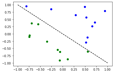
Primero, mostramos cómo TorchConnector permite entrenar una NeuralNetwork Cuántica para resolver tareas de clasificación utilizando el motor de diferenciación automática de PyTorch. Para ilustrar esto, realizaremos una clasificación binaria en un conjunto de datos generado aleatoriamente.
[2]:
# Generate random dataset

# Select dataset dimension (num_inputs) and size (num_samples)
num_inputs = 2
num_samples = 20

# Generate random input coordinates (X) and binary labels (y)
X = 2 * algorithm_globals.random.random([num_samples, num_inputs]) - 1
y01 = 1 * (np.sum(X, axis=1) >= 0)  # in { 0,  1}, y01 will be used for SamplerQNN example
y = 2 * y01 - 1  # in {-1, +1}, y will be used for EstimatorQNN example

# Convert to torch Tensors
X_ = Tensor(X)
y01_ = Tensor(y01).reshape(len(y)).long()
y_ = Tensor(y).reshape(len(y), 1)

# Plot dataset
for x, y_target in zip(X, y):
    if y_target == 1:
        plt.plot(x[0], x[1], "bo")
    else:
        plt.plot(x[0], x[1], "go")
plt.plot([-1, 1], [1, -1], "--", color="black")
plt.show()
A. Clasificación con PyTorch y EstimatorQNN#
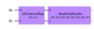
Vincular un EstimatorQNN a PyTorch es relativamente sencillo. Aquí ilustramos esto usando el EstimatorQNN construido a partir de un mapa de características y un ansatz.
[3]:
# Set up a circuit
feature_map = ZZFeatureMap(num_inputs)
ansatz = RealAmplitudes(num_inputs)
qc = QuantumCircuit(num_inputs)
qc.compose(feature_map, inplace=True)
qc.compose(ansatz, inplace=True)
qc.draw("mpl")
[3]:
[4]:
# Setup QNN
qnn1 = EstimatorQNN(
    circuit=qc, input_params=feature_map.parameters, weight_params=ansatz.parameters
)

# Set up PyTorch module
# Note: If we don't explicitly declare the initial weights
# they are chosen uniformly at random from [-1, 1].
initial_weights = 0.1 * (2 * algorithm_globals.random.random(qnn1.num_weights) - 1)
model1 = TorchConnector(qnn1, initial_weights=initial_weights)
print("Initial weights: ", initial_weights)
Initial weights:  [-0.01256962  0.06653564  0.04005302 -0.03752667  0.06645196  0.06095287
 -0.02250432 -0.04233438]
[5]:
# Test with a single input
model1(X_[0, :])
[5]:
tensor([-0.3285], grad_fn=<_TorchNNFunctionBackward>)
Optimizador#
La elección del optimizador para entrenar cualquier modelo de machine learning puede ser crucial para determinar el éxito del resultado de nuestro entrenamiento. Cuando usamos TorchConnector, obtenemos acceso a todos los algoritmos del optimizador definidos en el paquete [torch.optim] (enlace). Algunos de los algoritmos más famosos utilizados en las arquitecturas de machine learning populares incluyen Adam, SGD, o Adagrad. Sin embargo, para este tutorial usaremos el algoritmo L-BFGS (torch.optim.LBFGS), uno de los algoritmos de optimización de segundo orden más conocidos para la optimización numérica.
Función de Pérdida#
En cuanto a la función de pérdida, también podemos aprovechar los módulos predefinidos de PyTorch desde torch.nn, como las pérdidas Cross-Entropy o Mean Squared Error.
💡 Aclaración: En machine learning clásico, la regla general es aplicar una pérdida de entropía cruzada (Cross-Entropy) a las tareas de clasificación y una pérdida de MSE a las tareas de regresión. Sin embargo, esta recomendación se da bajo el supuesto de que la salida de la red de clasificación es un valor de probabilidad de clase en el rango EstimatorQNN no incluye dicha capa, y no aplicamos ningún mapeo a la salida (la siguiente sección muestra un ejemplo de aplicación de mapeo de paridad con SamplerQNNs), la salida de la QNN puede tomar cualquier valor en el rango
[6]:
# Define optimizer and loss
optimizer = LBFGS(model1.parameters())
f_loss = MSELoss(reduction="sum")

# Start training
model1.train()  # set model to training mode


# Note from (https://pytorch.org/docs/stable/optim.html):
# Some optimization algorithms such as LBFGS need to
# reevaluate the function multiple times, so you have to
# pass in a closure that allows them to recompute your model.
# The closure should clear the gradients, compute the loss,
# and return it.
def closure():
    optimizer.zero_grad()  # Initialize/clear gradients
    loss = f_loss(model1(X_), y_)  # Evaluate loss function
    loss.backward()  # Backward pass
    print(loss.item())  # Print loss
    return loss


# Run optimizer step4
optimizer.step(closure)
25.535646438598633
22.696760177612305
20.039228439331055
19.687908172607422
19.267208099365234
19.025373458862305
18.154708862304688
17.337854385375977
19.082578659057617
17.073287963867188
16.21839141845703
14.992582321166992
14.929339408874512
14.914533615112305
14.907636642456055
14.902364730834961
14.902134895324707
14.90211009979248
14.902111053466797
[6]:
tensor(25.5356, grad_fn=<MseLossBackward0>)
[7]:
# Evaluate model and compute accuracy
model1.eval()
y_predict = []
for x, y_target in zip(X, y):
    output = model1(Tensor(x))
    y_predict += [np.sign(output.detach().numpy())[0]]

print("Accuracy:", sum(y_predict == y) / len(y))

# Plot results
# red == wrongly classified
for x, y_target, y_p in zip(X, y, y_predict):
    if y_target == 1:
        plt.plot(x[0], x[1], "bo")
    else:
        plt.plot(x[0], x[1], "go")
    if y_target != y_p:
        plt.scatter(x[0], x[1], s=200, facecolors="none", edgecolors="r", linewidths=2)
plt.plot([-1, 1], [1, -1], "--", color="black")
plt.show()
Accuracy: 0.8
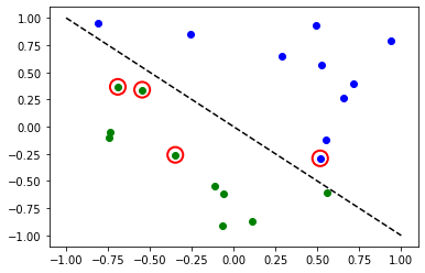
Los círculos rojos indican puntos de datos clasificados incorrectamente.
B. Clasificación con PyTorch y SamplerQNN#
Vincular una SamplerQNN``a PyTorch requiere un poco más de atención que con ``EstimatorQNN. Sin la configuración correcta, la propagación hacia atrás (backpropagation) no es posible.
En particular, debemos asegurarnos de que estamos devolviendo un arreglo denso de probabilidades en el paso hacia adelante de la red (sparse=False). Este parámetro está configurado en False de forma predeterminada, por lo que solo debemos asegurarnos de que no haya sido modificado.
⚠️ Atención: Si definimos una función de interpretación personalizada (en el ejemplo: parity), debemos recordar proporcionar explícitamente la forma de salida deseada (en el ejemplo: 2). Para obtener más información sobre la configuración inicial de parámetros para SamplerQNN, consulta la documentación oficial de qiskit.
[8]:
# Define feature map and ansatz
feature_map = ZZFeatureMap(num_inputs)
ansatz = RealAmplitudes(num_inputs, entanglement="linear", reps=1)

# Define quantum circuit of num_qubits = input dim
# Append feature map and ansatz
qc = QuantumCircuit(num_inputs)
qc.compose(feature_map, inplace=True)
qc.compose(ansatz, inplace=True)

# Define SamplerQNN and initial setup
parity = lambda x: "{:b}".format(x).count("1") % 2  # optional interpret function
output_shape = 2  # parity = 0, 1
qnn2 = SamplerQNN(
    circuit=qc,
    input_params=feature_map.parameters,
    weight_params=ansatz.parameters,
    interpret=parity,
    output_shape=output_shape,
)

# Set up PyTorch module
# Reminder: If we don't explicitly declare the initial weights
# they are chosen uniformly at random from [-1, 1].
initial_weights = 0.1 * (2 * algorithm_globals.random.random(qnn2.num_weights) - 1)
print("Initial weights: ", initial_weights)
model2 = TorchConnector(qnn2, initial_weights)
Initial weights: [ 0.0364991 -0.0720495 -0.06001836 -0.09852755]
Para obtener un recordatorio sobre el optimizador y las opciones de funciones de pérdida, puedes volver a esta sección.
[9]:
# Define model, optimizer, and loss
optimizer = LBFGS(model2.parameters())
f_loss = CrossEntropyLoss()  # Our output will be in the [0,1] range

# Start training
model2.train()

# Define LBFGS closure method (explained in previous section)
def closure():
    optimizer.zero_grad(set_to_none=True)  # Initialize gradient
    loss = f_loss(model2(X_), y01_)  # Calculate loss
    loss.backward()  # Backward pass

    print(loss.item())  # Print loss
    return loss


# Run optimizer (LBFGS requires closure)
optimizer.step(closure);
0.6925069093704224
0.6881508231163025
0.6516683101654053
0.6485998034477234
0.6394743919372559
0.7057444453239441
0.669085681438446
0.766187310218811
0.7188469171524048
0.7919709086418152
0.7598814964294434
0.7028256058692932
0.7486447095870972
0.6890242695808411
0.7760348916053772
0.7892935276031494
0.7556288242340088
0.7058126330375671
0.7203161716461182
0.7030722498893738
[10]:
# Evaluate model and compute accuracy
model2.eval()
y_predict = []
for x in X:
    output = model2(Tensor(x))
    y_predict += [np.argmax(output.detach().numpy())]

print("Accuracy:", sum(y_predict == y01) / len(y01))

# plot results
# red == wrongly classified
for x, y_target, y_ in zip(X, y01, y_predict):
    if y_target == 1:
        plt.plot(x[0], x[1], "bo")
    else:
        plt.plot(x[0], x[1], "go")
    if y_target != y_:
        plt.scatter(x[0], x[1], s=200, facecolors="none", edgecolors="r", linewidths=2)
plt.plot([-1, 1], [1, -1], "--", color="black")
plt.show()
Accuracy: 0.5
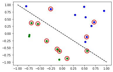
Los círculos rojos indican puntos de datos clasificados incorrectamente.
2. Regresión#
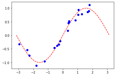
Usamos un modelo basado en la EstimatorQNN para ilustrar también cómo realizar una tarea de regresión. El conjunto de datos elegido en este caso se genera aleatoriamente siguiendo una onda sinusoidal.
[11]:
# Generate random dataset

num_samples = 20
eps = 0.2
lb, ub = -np.pi, np.pi
f = lambda x: np.sin(x)

X = (ub - lb) * algorithm_globals.random.random([num_samples, 1]) + lb
y = f(X) + eps * (2 * algorithm_globals.random.random([num_samples, 1]) - 1)
plt.plot(np.linspace(lb, ub), f(np.linspace(lb, ub)), "r--")
plt.plot(X, y, "bo")
plt.show()
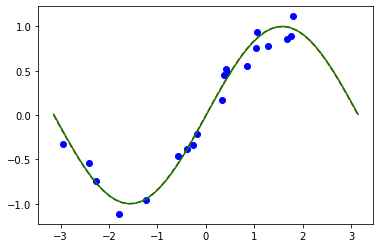
A. Regresión con PyTorch y EstimatorQNN#
La definición de la red y el ciclo de entrenamiento serán análogos a los de la tarea de clasificación usando EstimatorQNN. En este caso, definimos nuestro propio mapa de características y ansatz, pero hagámoslo un poco diferente.
[12]:
# Construct simple feature map
param_x = Parameter("x")
feature_map = QuantumCircuit(1, name="fm")
feature_map.ry(param_x, 0)

# Construct simple parameterized ansatz
param_y = Parameter("y")
ansatz = QuantumCircuit(1, name="vf")
ansatz.ry(param_y, 0)

qc = QuantumCircuit(1)
qc.compose(feature_map, inplace=True)
qc.compose(ansatz, inplace=True)

# Construct QNN
qnn3 = EstimatorQNN(circuit=qc, input_params=[param_x], weight_params=[param_y])

# Set up PyTorch module
# Reminder: If we don't explicitly declare the initial weights
# they are chosen uniformly at random from [-1, 1].
initial_weights = 0.1 * (2 * algorithm_globals.random.random(qnn3.num_weights) - 1)
model3 = TorchConnector(qnn3, initial_weights)
Para obtener un recordatorio sobre el optimizador y las opciones de funciones de pérdida, puedes volver a esta sección.
[13]:
# Define optimizer and loss function
optimizer = LBFGS(model3.parameters())
f_loss = MSELoss(reduction="sum")

# Start training
model3.train()  # set model to training mode

# Define objective function
def closure():
    optimizer.zero_grad(set_to_none=True)  # Initialize gradient
    loss = f_loss(model3(Tensor(X)), Tensor(y))  # Compute batch loss
    loss.backward()  # Backward pass
    print(loss.item())  # Print loss
    return loss


# Run optimizer
optimizer.step(closure)
14.947757720947266
2.948650360107422
8.952412605285645
0.37905153632164
0.24995625019073486
0.2483610212802887
0.24835753440856934
[13]:
tensor(14.9478, grad_fn=<MseLossBackward0>)
[14]:
# Plot target function
plt.plot(np.linspace(lb, ub), f(np.linspace(lb, ub)), "r--")

# Plot data
plt.plot(X, y, "bo")

# Plot fitted line
model3.eval()
y_ = []
for x in np.linspace(lb, ub):
    output = model3(Tensor([x]))
    y_ += [output.detach().numpy()[0]]
plt.plot(np.linspace(lb, ub), y_, "g-")
plt.show()
Parte 2: Clasificación MNIST, QNNs Híbridas#
En esta segunda parte, mostramos cómo aprovechar una red neuronal híbrida cuántica-clásica utilizando TorchConnector, para realizar una tarea de clasificación de imágenes más compleja en el conjunto de datos de dígitos manuscritos del MNIST.
Para obtener una explicación más detallada (pre-TorchConnector) sobre las redes neuronales híbridas cuánticas-clásicas, puedes consultar la sección correspondiente en el Libro de texto de Qiskit.
[15]:
# Additional torch-related imports
import torch
from torch import cat, no_grad, manual_seed
from torch.utils.data import DataLoader
from torchvision import datasets, transforms
import torch.optim as optim
from torch.nn import (
    Module,
    Conv2d,
    Linear,
    Dropout2d,
    NLLLoss,
    MaxPool2d,
    Flatten,
    Sequential,
    ReLU,
)
import torch.nn.functional as F
Paso 1: Definición de cargadores de datos para entrenamiento y prueba#
Aprovechamos la API de torchvision para cargar directamente un subconjunto del conjunto de datos MNIST y definir los DataLoaders de torch (enlace) para entrenar y probar.
[16]:
# Train Dataset
# -------------

# Set train shuffle seed (for reproducibility)
manual_seed(42)

batch_size = 1
n_samples = 100  # We will concentrate on the first 100 samples

# Use pre-defined torchvision function to load MNIST train data
X_train = datasets.MNIST(
    root="./data", train=True, download=True, transform=transforms.Compose([transforms.ToTensor()])
)

# Filter out labels (originally 0-9), leaving only labels 0 and 1
idx = np.append(
    np.where(X_train.targets == 0)[0][:n_samples], np.where(X_train.targets == 1)[0][:n_samples]
)
X_train.data = X_train.data[idx]
X_train.targets = X_train.targets[idx]

# Define torch dataloader with filtered data
train_loader = DataLoader(X_train, batch_size=batch_size, shuffle=True)
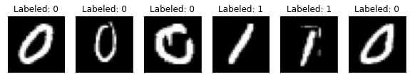
Si realizamos una visualización rápida, podemos ver que el conjunto de datos de entrenamiento consta de imágenes de 0s y 1s escritos a mano.
[17]:
n_samples_show = 6

data_iter = iter(train_loader)
fig, axes = plt.subplots(nrows=1, ncols=n_samples_show, figsize=(10, 3))

while n_samples_show > 0:
    images, targets = data_iter.__next__()

    axes[n_samples_show - 1].imshow(images[0, 0].numpy().squeeze(), cmap="gray")
    axes[n_samples_show - 1].set_xticks([])
    axes[n_samples_show - 1].set_yticks([])
    axes[n_samples_show - 1].set_title("Labeled: {}".format(targets[0].item()))

    n_samples_show -= 1
[18]:
# Test Dataset
# -------------

# Set test shuffle seed (for reproducibility)
# manual_seed(5)

n_samples = 50

# Use pre-defined torchvision function to load MNIST test data
X_test = datasets.MNIST(
    root="./data", train=False, download=True, transform=transforms.Compose([transforms.ToTensor()])
)

# Filter out labels (originally 0-9), leaving only labels 0 and 1
idx = np.append(
    np.where(X_test.targets == 0)[0][:n_samples], np.where(X_test.targets == 1)[0][:n_samples]
)
X_test.data = X_test.data[idx]
X_test.targets = X_test.targets[idx]

# Define torch dataloader with filtered data
test_loader = DataLoader(X_test, batch_size=batch_size, shuffle=True)
Paso 2: Definición del Modelo Híbrido y de la QNN#
Este segundo paso muestra el poder del TorchConnector. Después de definir nuestra capa de red neuronal cuántica (en este caso, una EstimatorQNN), podemos incrustarla en una capa en nuestro Module de torch, al inicializar un conector torch como TorchConnector(qnn).
⚠️ Atención: Para tener un gradiente de propagación hacia atrás (backpropagation) adecuado en modelos híbridos, DEBEMOS establecer el parámetro inicial input_gradients en TRUE durante la inicialización de la qnn.
[19]:
# Define and create QNN
def create_qnn():
    feature_map = ZZFeatureMap(2)
    ansatz = RealAmplitudes(2, reps=1)
    qc = QuantumCircuit(2)
    qc.compose(feature_map, inplace=True)
    qc.compose(ansatz, inplace=True)

    # REMEMBER TO SET input_gradients=True FOR ENABLING HYBRID GRADIENT BACKPROP
    qnn = EstimatorQNN(
        circuit=qc,
        input_params=feature_map.parameters,
        weight_params=ansatz.parameters,
        input_gradients=True,
    )
    return qnn


qnn4 = create_qnn()
[20]:
# Define torch NN module


class Net(Module):
    def __init__(self, qnn):
        super().__init__()
        self.conv1 = Conv2d(1, 2, kernel_size=5)
        self.conv2 = Conv2d(2, 16, kernel_size=5)
        self.dropout = Dropout2d()
        self.fc1 = Linear(256, 64)
        self.fc2 = Linear(64, 2)  # 2-dimensional input to QNN
        self.qnn = TorchConnector(qnn)  # Apply torch connector, weights chosen
        # uniformly at random from interval [-1,1].
        self.fc3 = Linear(1, 1)  # 1-dimensional output from QNN

    def forward(self, x):
        x = F.relu(self.conv1(x))
        x = F.max_pool2d(x, 2)
        x = F.relu(self.conv2(x))
        x = F.max_pool2d(x, 2)
        x = self.dropout(x)
        x = x.view(x.shape[0], -1)
        x = F.relu(self.fc1(x))
        x = self.fc2(x)
        x = self.qnn(x)  # apply QNN
        x = self.fc3(x)
        return cat((x, 1 - x), -1)


model4 = Net(qnn4)
Paso 3: Entrenamiento#
[21]:
# Define model, optimizer, and loss function
optimizer = optim.Adam(model4.parameters(), lr=0.001)
loss_func = NLLLoss()

# Start training
epochs = 10  # Set number of epochs
loss_list = []  # Store loss history
model4.train()  # Set model to training mode

for epoch in range(epochs):
    total_loss = []
    for batch_idx, (data, target) in enumerate(train_loader):
        optimizer.zero_grad(set_to_none=True)  # Initialize gradient
        output = model4(data)  # Forward pass
        loss = loss_func(output, target)  # Calculate loss
        loss.backward()  # Backward pass
        optimizer.step()  # Optimize weights
        total_loss.append(loss.item())  # Store loss
    loss_list.append(sum(total_loss) / len(total_loss))
    print("Training [{:.0f}%]\tLoss: {:.4f}".format(100.0 * (epoch + 1) / epochs, loss_list[-1]))
Training [10%]  Loss: -1.1630
Training [20%]  Loss: -1.5294
Training [30%]  Loss: -1.7855
Training [40%]  Loss: -1.9863
Training [50%]  Loss: -2.2257
Training [60%]  Loss: -2.4513
Training [70%]  Loss: -2.6758
Training [80%]  Loss: -2.8832
Training [90%]  Loss: -3.1006
Training [100%] Loss: -3.3061
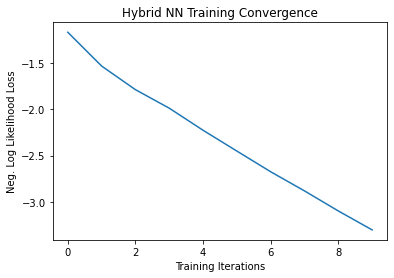
[22]:
# Plot loss convergence
plt.plot(loss_list)
plt.title("Hybrid NN Training Convergence")
plt.xlabel("Training Iterations")
plt.ylabel("Neg. Log Likelihood Loss")
plt.show()
Ahora guardaremos el modelo entrenado, solo para mostrar cómo se puede guardar un modelo híbrido y reutilizarlo más tarde para la inferencia. Para guardar y cargar modelos híbridos, al usar TorchConnector, sigue las recomendaciones de PyTorch para guardar y cargar los modelos.
[23]:
torch.save(model4.state_dict(), "model4.pt")
Paso 4: Evaluación#
Partimos de recrear el modelo y cargar el estado desde el archivo previamente guardado. Creaste una capa QNN usando otro simulador o un hardware real. Por lo tanto, puedes entrenar un modelo en hardware real disponible en la nube y luego, para la inferencia, usar un simulador o viceversa. En aras de la simplicidad, creamos una nueva red neuronal cuántica de la misma manera que arriba.
[24]:
qnn5 = create_qnn()
model5 = Net(qnn5)
model5.load_state_dict(torch.load("model4.pt"))
[24]:
<All keys matched successfully>
[25]:
model5.eval()  # set model to evaluation mode
with no_grad():

    correct = 0
    for batch_idx, (data, target) in enumerate(test_loader):
        output = model5(data)
        if len(output.shape) == 1:
            output = output.reshape(1, *output.shape)

        pred = output.argmax(dim=1, keepdim=True)
        correct += pred.eq(target.view_as(pred)).sum().item()

        loss = loss_func(output, target)
        total_loss.append(loss.item())

    print(
        "Performance on test data:\n\tLoss: {:.4f}\n\tAccuracy: {:.1f}%".format(
            sum(total_loss) / len(total_loss), correct / len(test_loader) / batch_size * 100
        )
    )
Performance on test data:
        Loss: -3.3585
        Accuracy: 100.0%
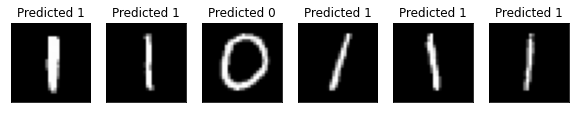
[26]:
# Plot predicted labels

n_samples_show = 6
count = 0
fig, axes = plt.subplots(nrows=1, ncols=n_samples_show, figsize=(10, 3))

model5.eval()
with no_grad():
    for batch_idx, (data, target) in enumerate(test_loader):
        if count == n_samples_show:
            break
        output = model5(data[0:1])
        if len(output.shape) == 1:
            output = output.reshape(1, *output.shape)

        pred = output.argmax(dim=1, keepdim=True)

        axes[count].imshow(data[0].numpy().squeeze(), cmap="gray")

        axes[count].set_xticks([])
        axes[count].set_yticks([])
        axes[count].set_title("Predicted {}".format(pred.item()))

        count += 1
🎉🎉🎉🎉 Ahora puedes experimentar con tus propios conjuntos de datos y arquitecturas híbridas utilizando Qiskit Machine Learning. ¡Buena suerte!
[27]:
import qiskit.tools.jupyter

%qiskit_version_table
%qiskit_copyright
Version Information
| Qiskit Software | Version |
|---|---|
qiskit-terra | 0.22.0 |
qiskit-aer | 0.11.1 |
qiskit-ignis | 0.7.0 |
qiskit | 0.33.0 |
qiskit-machine-learning | 0.5.0 |
| System information | |
| Python version | 3.7.9 |
| Python compiler | MSC v.1916 64 bit (AMD64) |
| Python build | default, Aug 31 2020 17:10:11 |
| OS | Windows |
| CPUs | 4 |
| Memory (Gb) | 31.837730407714844 |
| Thu Nov 03 09:57:38 2022 GMT Standard Time | |
This code is a part of Qiskit
© Copyright IBM 2017, 2022.
This code is licensed under the Apache License, Version 2.0. You may
obtain a copy of this license in the LICENSE.txt file in the root directory
of this source tree or at http://www.apache.org/licenses/LICENSE-2.0.
Any modifications or derivative works of this code must retain this
copyright notice, and modified files need to carry a notice indicating
that they have been altered from the originals.