Note
This page was generated from tut//4-Analysis//4.22-Eigenmode-matrix.ipynb.
Sweeps - Eigenmode matrix#
Prerequisite#
You need to have a working local installation of Ansys
1. Perform the necessary imports and create a QDesign in Metal first.#
[1]:
%load_ext autoreload
%autoreload 2
[2]:
import qiskit_metal as metal
from qiskit_metal import designs, draw
from qiskit_metal import MetalGUI, Dict, Headings
from qiskit_metal.analyses.quantization import EPRanalysis
[3]:
# Create the design in Metal
# Create a design by specifying the chip size and open Metal GUI.

design = designs.DesignPlanar({}, True)
design.chips.main.size['size_x'] = '2mm'
design.chips.main.size['size_y'] = '2mm'

gui = MetalGUI(design)

from qiskit_metal.qlibrary.qubits.transmon_pocket import TransmonPocket
from qiskit_metal.qlibrary.terminations.open_to_ground import OpenToGround
from qiskit_metal.qlibrary.tlines.meandered import RouteMeander
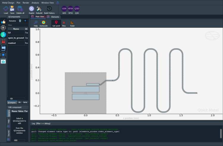
In this example, the design consists of 1 qubit and 1 CPW connected to OpenToGround.#
[4]:
# Allow running the same cell here multiple times to overwrite changes
design.overwrite_enabled = True

# Remove all qcomponents from GUI.
design.delete_all_components()

# So as to demonstrate the quality factor outputs easily, the
#subtrate material type is being changed to FR4_epoxy from the
#default of silicon
design.chips.main.material = 'FR4_epoxy'

q1 = TransmonPocket(
    design,
    'Q1',
    options=dict(pad_width='425 um',
                 pocket_height='650um',
                 hfss_inductance = '17nH',
                 connection_pads=dict(
                     readout=dict(loc_W=+1, loc_H=+1, pad_width='200um'))))
otg = OpenToGround(design,
                   'open_to_ground',
                   options=dict(pos_x='1.75mm', pos_y='0um', orientation='0'))
readout = RouteMeander(
    design, 'readout',
    Dict(
        total_length='6 mm',
        hfss_wire_bonds = True,
        fillet='90 um',
        lead=dict(start_straight='100um'),
        pin_inputs=Dict(start_pin=Dict(component='Q1', pin='readout'),
                        end_pin=Dict(component='open_to_ground', pin='open')),
    ))

gui.rebuild()
gui.autoscale()
[5]:
gui.screenshot()
2 Metal passes information to ‘hfss’ simulator, and gets a solution matrix.#
[6]:
# Create a separate analysis object for the combined qbit+readout.
eig_qres = EPRanalysis(design, "hfss")
Prepare data to pass as arguments for method run_sweep().
Method run_sweep() will open the simulation software if software is not open already.
[7]:
### for render_design()
# Render every QComponent in QDesign.
render_qcomps = []

# Identify which kind of pins in Ansys.
# Follow details from renderer in
# QHFSSRenderer.render_design.
# No pins are open, so don't need to utilize render_endcaps.
open_terminations = []

#List of tuples of jj's that shouldn't be rendered.
#Follow details from renderer in QHFSSRenderer.render_design.
render_ignored_jjs = []

# Either calculate a bounding box based on the location of
# rendered geometries or use chip size from design class.
box_plus_buffer = True
[8]:
# For simulator hfss, the setup options are :
# min_freq_ghz, n_modes, max_delta_f, max_passes, min_passes, min_converged=None,
# pct_refinement, basis_order

# If you don't pass all the arguments, the default is determined by
# QHFSSRenderer's default_options.

# If a setup named "sweeper_em_setup" exists in the project, it will be deleted,
# and a new setup will be added.

eig_qres.sim.setup.name="sweeper_em_setup"
eig_qres.sim.setup.min_freq_ghz=4
eig_qres.sim.setup.n_modes=2
eig_qres.sim.setup.max_passes=15
eig_qres.sim.setup.min_converged = 2
eig_qres.sim.setup.max_delta_f = 0.2

eig_qres.setup.junctions.jj.rect = 'JJ_rect_Lj_Q1_rect_jj'
eig_qres.setup.junctions.jj.line = 'JJ_Lj_Q1_rect_jj_'
Connect to Ansys HFSS, eigenmode solution.
Rebuild QComponents in Metal.
Render QComponents within HFSS and setup.
Delete/Clear the HFSS between each calculation of solution matrix.
Calculate solution matrix for each value in option_sweep.
Return a dict and return code. If the return code is zero, there were no errors detected.#
The dict has: key = each value used to sweep, value = data from simulators#
This could take minutes based size of design.#
[9]:
#Note: The method will connect to Ansys, activate_eigenmode_design(), add_eigenmode_setup().

all_sweeps, return_code = eig_qres.run_sweep(readout.name,
                                        'total_length',
                                        ['10mm', '11mm', '12mm'],
                                        render_qcomps,
                                        open_terminations,
                                         ignored_jjs=render_ignored_jjs,
                                        design_name="GetEigenModeSolution",
                                       box_plus_buffer=box_plus_buffer
                                      )
INFO 08:11AM [connect_project]: Connecting to Ansys Desktop API...
INFO 08:11AM [load_ansys_project]:      Opened Ansys App
INFO 08:11AM [load_ansys_project]:      Opened Ansys Desktop v2020.2.0
INFO 08:11AM [load_ansys_project]:      Opened Ansys Project
        Folder:    C:/Ansoft/
        Project:   Project23
INFO 08:11AM [connect_design]: No active design found (or error getting active design).
INFO 08:11AM [connect]:          Connected to project "Project23". No design detected
INFO 08:11AM [connect_design]:  Opened active design
        Design:    GetEigenModeSolution_hfss [Solution type: Eigenmode]
WARNING 08:11AM [connect_setup]:        No design setup detected.
WARNING 08:11AM [connect_setup]:        Creating eigenmode default setup.
INFO 08:11AM [get_setup]:       Opened setup `Setup`  (<class 'pyEPR.ansys.HfssEMSetup'>)
INFO 08:11AM [get_setup]:       Opened setup `sweeper_em_setup`  (<class 'pyEPR.ansys.HfssEMSetup'>)
INFO 08:11AM [analyze]: Analyzing setup sweeper_em_setup
08:26AM 34s INFO [get_f_convergence]: Saved convergences to C:\workspace\qiskit-metal\docs\tut\4-Analysis\hfss_eig_f_convergence.csv
Design "GetEigenModeSolution_hfss" info:
        # eigenmodes    2
        # variations    1
Design "GetEigenModeSolution_hfss" info:
        # eigenmodes    2
        # variations    1

        energy_elec_all       = 5.19788159957566e-25
        energy_elec_substrate = 4.2287113157029e-25
        EPR of substrate = 81.4%

        energy_mag    = 8.01738203686217e-27
        energy_mag % of energy_elec_all  = 1.5%


Variation 0  [1/1]

  Mode 0 at 7.53 GHz   [1/2]
    Calculating ℰ_magnetic,ℰ_electric
       (ℰ_E-ℰ_H)/ℰ_E       ℰ_E       ℰ_H
               98.5%  2.599e-25 4.009e-27

    Calculating junction energy participation ration (EPR)
        method=`line_voltage`. First estimates:
        junction        EPR p_0j   sign s_0j    (p_capacitive)
                Energy fraction (Lj over Lj&Cj)= 95.71%
        jj                1.6736  (+)        0.0750176
                (U_tot_cap-U_tot_ind)/mean=-22.21%
WARNING: This simulation must not have converged well!!!                The difference in the total cap and ind energies is larger than 10%.                Proceed with caution.
Calculating Qdielectric_main for mode 0 (0/1)
p_dielectric_main_0 = 0.8135451403987578

  Mode 1 at 8.86 GHz   [2/2]
    Calculating ℰ_magnetic,ℰ_electric
       (ℰ_E-ℰ_H)/ℰ_E       ℰ_E       ℰ_H
                1.2%  5.877e-25 5.809e-25

    Calculating junction energy participation ration (EPR)
        method=`line_voltage`. First estimates:
        junction        EPR p_1j   sign s_1j    (p_capacitive)
                Energy fraction (Lj over Lj&Cj)= 94.17%
        jj              0.0199851  (+)        0.00123759
                (U_tot_cap-U_tot_ind)/mean=-0.36%
Calculating Qdielectric_main for mode 1 (1/1)
p_dielectric_main_1 = 0.8119553568702682
WARNING 08:27AM [__init__]: <p>Error: <class 'IndexError'></p>
ERROR 08:27AM [_get_participation_normalized]: WARNING: U_tot_cap-U_tot_ind / mean = 44.4% is > 15%.
Is the simulation converged? Proceed with caution
ANALYSIS DONE. Data saved to:

C:\data-pyEPR\Project23\GetEigenModeSolution_hfss\2021-08-18 08-26-35.npz


         Differences in variations:


 . . . . . . . . . . . . . . . . . . . . . . . . . . . . . . . . . . . . . . . .
Variation 0

Starting the diagonalization
ERROR 08:27AM [_get_participation_normalized]: WARNING: U_tot_cap-U_tot_ind / mean = 44.4% is > 15%.
Is the simulation converged? Proceed with caution
Finished the diagonalization
Pm_norm=
modes
0    0.635168
1    0.817290
dtype: float64

Pm_norm idx =
      jj
0   True
1  False
*** P (participation matrix, not normlz.)
         jj
0  1.556815
1  0.019960

*** S (sign-bit matrix)
   s_jj
0     1
1     1
*** P (participation matrix, normalized.)
      0.99
      0.02

*** Chi matrix O1 PT (MHz)
    Diag is anharmonicity, off diag is full cross-Kerr.
       424     20.1
      20.1    0.239

*** Chi matrix ND (MHz)
       499     10.1
      10.1   0.0723

*** Frequencies O1 PT (MHz)
0    7100.043062
1    8845.729528
dtype: float64

*** Frequencies ND (MHz)
0    7067.159806
1    8847.889665
dtype: float64

*** Q_coupling
Empty DataFrame
Columns: []
Index: [0, 1]
Mode frequencies (MHz)#
Numerical diagonalization
| Lj | 10 |
|---|---|
| eigenmode | |
| 0 | 7100.04 |
| 1 | 8845.73 |
Kerr Non-linear coefficient table (MHz)#
Numerical diagonalization
| 0 | 1 | ||
|---|---|---|---|
| Lj | |||
| 10 | 0 | 498.59 | 10.14 |
| 1 | 10.14 | 0.07 |
INFO 08:27AM [connect_design]:  Opened active design
        Design:    GetEigenModeSolution_hfss [Solution type: Eigenmode]
INFO 08:27AM [get_setup]:       Opened setup `sweeper_em_setup`  (<class 'pyEPR.ansys.HfssEMSetup'>)
INFO 08:27AM [analyze]: Analyzing setup sweeper_em_setup
08:36AM 21s INFO [get_f_convergence]: Saved convergences to C:\workspace\qiskit-metal\docs\tut\4-Analysis\hfss_eig_f_convergence.csv
Design "GetEigenModeSolution_hfss" info:
        # eigenmodes    2
        # variations    1
Design "GetEigenModeSolution_hfss" info:
        # eigenmodes    2
        # variations    1

        energy_elec_all       = 1.24548064887814e-24
        energy_elec_substrate = 1.01220397065148e-24
        EPR of substrate = 81.3%

        energy_mag    = 6.56191412175113e-26
        energy_mag % of energy_elec_all  = 5.3%


Variation 0  [1/1]

  Mode 0 at 7.47 GHz   [1/2]
    Calculating ℰ_magnetic,ℰ_electric
       (ℰ_E-ℰ_H)/ℰ_E       ℰ_E       ℰ_H
               94.7%  6.227e-25 3.281e-26

    Calculating junction energy participation ration (EPR)
        method=`line_voltage`. First estimates:
        junction        EPR p_0j   sign s_0j    (p_capacitive)
                Energy fraction (Lj over Lj&Cj)= 95.78%
        jj               1.61044  (+)        0.0709035
                (U_tot_cap-U_tot_ind)/mean=-21.66%
WARNING: This simulation must not have converged well!!!                The difference in the total cap and ind energies is larger than 10%.                Proceed with caution.
Calculating Qdielectric_main for mode 0 (0/1)
p_dielectric_main_0 = 0.8127014832090866

  Mode 1 at 8.07 GHz   [2/2]
    Calculating ℰ_magnetic,ℰ_electric
       (ℰ_E-ℰ_H)/ℰ_E       ℰ_E       ℰ_H
                4.9%  7.606e-25 7.235e-25

    Calculating junction energy participation ration (EPR)
        method=`line_voltage`. First estimates:
        junction        EPR p_1j   sign s_1j    (p_capacitive)
                Energy fraction (Lj over Lj&Cj)= 95.11%
        jj              0.0831536  (+)        0.00427873
                (U_tot_cap-U_tot_ind)/mean=-1.48%
Calculating Qdielectric_main for mode 1 (1/1)
p_dielectric_main_1 = 0.8110869059274507
WARNING 08:36AM [__init__]: <p>Error: <class 'IndexError'></p>
ERROR 08:36AM [_get_participation_normalized]: WARNING: U_tot_cap-U_tot_ind / mean = 43.3% is > 15%.
Is the simulation converged? Proceed with caution
ERROR 08:36AM [_get_participation_normalized]: WARNING: U_tot_cap-U_tot_ind / mean = 43.3% is > 15%.
Is the simulation converged? Proceed with caution
ANALYSIS DONE. Data saved to:

C:\data-pyEPR\Project23\GetEigenModeSolution_hfss\2021-08-18 08-36-22.npz


         Differences in variations:


 . . . . . . . . . . . . . . . . . . . . . . . . . . . . . . . . . . . . . . . .
Variation 0

Starting the diagonalization
Finished the diagonalization
Pm_norm=
modes
0    0.639346
1    0.806611
dtype: float64

Pm_norm idx =
      jj
0   True
1  False
*** P (participation matrix, not normlz.)
         jj
0  1.503817
1  0.082799

*** S (sign-bit matrix)
   s_jj
0     1
1     1
*** P (participation matrix, normalized.)
      0.96
     0.083

*** Chi matrix O1 PT (MHz)
    Diag is anharmonicity, off diag is full cross-Kerr.
       394     73.4
      73.4     3.42

*** Chi matrix ND (MHz)
       532     18.8
      18.8    0.297

*** Frequencies O1 PT (MHz)
0    7036.474625
1    8032.650030
dtype: float64

*** Frequencies ND (MHz)
0    6983.674726
1    8048.708620
dtype: float64

*** Q_coupling
Empty DataFrame
Columns: []
Index: [0, 1]
Mode frequencies (MHz)#
Numerical diagonalization
| Lj | 10 |
|---|---|
| eigenmode | |
| 0 | 7036.47 |
| 1 | 8032.65 |
Kerr Non-linear coefficient table (MHz)#
Numerical diagonalization
| 0 | 1 | ||
|---|---|---|---|
| Lj | |||
| 10 | 0 | 532.36 | 18.82 |
| 1 | 18.82 | 0.30 |
INFO 08:36AM [connect_design]:  Opened active design
        Design:    GetEigenModeSolution_hfss [Solution type: Eigenmode]
INFO 08:37AM [get_setup]:       Opened setup `sweeper_em_setup`  (<class 'pyEPR.ansys.HfssEMSetup'>)
INFO 08:37AM [analyze]: Analyzing setup sweeper_em_setup
08:49AM 07s INFO [get_f_convergence]: Saved convergences to C:\workspace\qiskit-metal\docs\tut\4-Analysis\hfss_eig_f_convergence.csv
Design "GetEigenModeSolution_hfss" info:
        # eigenmodes    2
        # variations    1
Design "GetEigenModeSolution_hfss" info:
        # eigenmodes    2
        # variations    1

        energy_elec_all       = 1.24148729817218e-24
        energy_elec_substrate = 1.00761523148401e-24
        EPR of substrate = 81.2%

        energy_mag    = 9.86581588344368e-25
        energy_mag % of energy_elec_all  = 79.5%


Variation 0  [1/1]

  Mode 0 at 7.33 GHz   [1/2]
    Calculating ℰ_magnetic,ℰ_electric
       (ℰ_E-ℰ_H)/ℰ_E       ℰ_E       ℰ_H
               20.5%  6.207e-25 4.933e-25

    Calculating junction energy participation ration (EPR)
        method=`line_voltage`. First estimates:
        junction        EPR p_0j   sign s_0j    (p_capacitive)
                Energy fraction (Lj over Lj&Cj)= 95.93%
        jj              0.349277  (+)        0.0148271
                (U_tot_cap-U_tot_ind)/mean=-5.98%
Calculating Qdielectric_main for mode 0 (0/1)
p_dielectric_main_0 = 0.8116194446511892

  Mode 1 at 7.62 GHz   [2/2]
    Calculating ℰ_magnetic,ℰ_electric
       (ℰ_E-ℰ_H)/ℰ_E       ℰ_E       ℰ_H
               79.1%  2.755e-25 5.769e-26

    Calculating junction energy participation ration (EPR)
        method=`line_voltage`. First estimates:
        junction        EPR p_1j   sign s_1j    (p_capacitive)
                Energy fraction (Lj over Lj&Cj)= 95.61%
        jj                1.3439  (+)        0.0616636
                (U_tot_cap-U_tot_ind)/mean=-18.80%
WARNING: This simulation must not have converged well!!!                The difference in the total cap and ind energies is larger than 10%.                Proceed with caution.
Calculating Qdielectric_main for mode 1 (1/1)
p_dielectric_main_1 = 0.8133632043452139
WARNING 08:49AM [__init__]: <p>Error: <class 'IndexError'></p>
ERROR 08:49AM [_get_participation_normalized]: WARNING: U_tot_cap-U_tot_ind / mean = 37.6% is > 15%.
Is the simulation converged? Proceed with caution
ERROR 08:49AM [_get_participation_normalized]: WARNING: U_tot_cap-U_tot_ind / mean = 37.6% is > 15%.
Is the simulation converged? Proceed with caution
ANALYSIS DONE. Data saved to:

C:\data-pyEPR\Project23\GetEigenModeSolution_hfss\2021-08-18 08-49-08.npz


         Differences in variations:


 . . . . . . . . . . . . . . . . . . . . . . . . . . . . . . . . . . . . . . . .
Variation 0

Starting the diagonalization
Finished the diagonalization
Pm_norm=
modes
0    0.766393
1    0.663454
dtype: float64

Pm_norm idx =
     jj
0  True
1  True
*** P (participation matrix, not normlz.)
         jj
0  0.344174
1  1.265842

*** S (sign-bit matrix)
   s_jj
0     1
1     1
*** P (participation matrix, normalized.)
      0.26
      0.84

*** Chi matrix O1 PT (MHz)
    Diag is anharmonicity, off diag is full cross-Kerr.
      28.6      189
       189      313

*** Chi matrix ND (MHz)
       526     -492
      -492      624

*** Frequencies O1 PT (MHz)
0    7209.141624
1    7215.058834
dtype: float64

*** Frequencies ND (MHz)
0    7432.783625
1    6939.798837
dtype: float64

*** Q_coupling
Empty DataFrame
Columns: []
Index: [0, 1]
Mode frequencies (MHz)#
Numerical diagonalization
| Lj | 10 |
|---|---|
| eigenmode | |
| 0 | 7209.14 |
| 1 | 7215.06 |
Kerr Non-linear coefficient table (MHz)#
Numerical diagonalization
| 0 | 1 | ||
|---|---|---|---|
| Lj | |||
| 10 | 0 | 526.43 | -492.01 |
| 1 | -492.01 | 624.37 |
[10]:
all_sweeps.keys()
[10]:
dict_keys(['10mm', '11mm', '12mm'])
[11]:
# For example, just one group of solution data.
all_sweeps['10mm'].keys()
[11]:
dict_keys(['option_name', 'variables', 'sim_variables'])
[12]:
all_sweeps['10mm']
[12]:
{'option_name': 'total_length',
 'variables': {'energy_elec': 5.19788159957566e-25,
  'energy_elec_sub': 4.2287113157029e-25,
  'energy_mag': 8.01738203686217e-27},
 'sim_variables': {'sim_setup_name': 'sweeper_em_setup',
  'convergence_t':              Solved Elements  Max Delta Freq. %
  Pass Number
  1                      12372                NaN
  2                      16089           46.90700
  3                      20923           26.83400
  4                      27201           12.39700
  5                      35009            5.13720
  6                      45251            3.05090
  7                      58833            1.58050
  8                      76494            1.37040
  9                      99448            0.75837
  10                    129285            0.63878
  11                    168080            0.27581
  12                    218509            0.35048
  13                    284068            0.39353
  14                    369273            0.37846
  15                    480014            0.23127,
  'convergence_f':          re(Mode(1)) [g]  re(Mode(2)) [g]
  Pass []
  1               5.569390        11.880396
  2               4.638777         6.307600
  3               5.883535         7.416275
  4               6.612905         7.967902
  5               6.952620         8.203356
  6               7.139302         8.453635
  7               7.252139         8.571936
  8               7.325233         8.689408
  9               7.365970         8.755306
  10              7.413022         8.793678
  11              7.433468         8.810855
  12              7.459521         8.825424
  13              7.488876         8.834471
  14              7.517219         8.844294
  15              7.534604         8.856040}}
[13]:
all_sweeps['10mm']['variables']
[13]:
{'energy_elec': 5.19788159957566e-25,
 'energy_elec_sub': 4.2287113157029e-25,
 'energy_mag': 8.01738203686217e-27}
[14]:
all_sweeps['10mm']['sim_variables']['convergence_t']
[14]:
| Solved Elements | Max Delta Freq. % | |
|---|---|---|
| Pass Number | ||
| 1 | 12372 | NaN |
| 2 | 16089 | 46.90700 |
| 3 | 20923 | 26.83400 |
| 4 | 27201 | 12.39700 |
| 5 | 35009 | 5.13720 |
| 6 | 45251 | 3.05090 |
| 7 | 58833 | 1.58050 |
| 8 | 76494 | 1.37040 |
| 9 | 99448 | 0.75837 |
| 10 | 129285 | 0.63878 |
| 11 | 168080 | 0.27581 |
| 12 | 218509 | 0.35048 |
| 13 | 284068 | 0.39353 |
| 14 | 369273 | 0.37846 |
| 15 | 480014 | 0.23127 |
[15]:
all_sweeps['10mm']['sim_variables']['convergence_f']
[15]:
| re(Mode(1)) [g] | re(Mode(2)) [g] | |
|---|---|---|
| Pass [] | ||
| 1 | 5.569390 | 11.880396 |
| 2 | 4.638777 | 6.307600 |
| 3 | 5.883535 | 7.416275 |
| 4 | 6.612905 | 7.967902 |
| 5 | 6.952620 | 8.203356 |
| 6 | 7.139302 | 8.453635 |
| 7 | 7.252139 | 8.571936 |
| 8 | 7.325233 | 8.689408 |
| 9 | 7.365970 | 8.755306 |
| 10 | 7.413022 | 8.793678 |
| 11 | 7.433468 | 8.810855 |
| 12 | 7.459521 | 8.825424 |
| 13 | 7.488876 | 8.834471 |
| 14 | 7.517219 | 8.844294 |
| 15 | 7.534604 | 8.856040 |
[16]:
# Uncomment the next close simulation software.
#eig_qres.sim.close()
[17]:
# Uncomment next line if you would like to close the gui
#gui.main_window.close()
For more information, review the Introduction to Quantum Computing and Quantum Hardware lectures below
|
Lecture Video | Lecture Notes | Lab |
|
Lecture Video | Lecture Notes | Lab |
|
Lecture Video | Lecture Notes | Lab |
|
Lecture Video | Lecture Notes | Lab |
|
Lecture Video | Lecture Notes | Lab |
|
Lecture Video | Lecture Notes | Lab |