Note
This page was generated from tut//4-Analysis//4.11-Analyze-and-tune-a-transmon.ipynb.
Analyzing and tuning a transmon qubit
We will showcase two methods (EPR amd LOM) to analyze the same design. Specifically, we will use here the advanced methods to run the simulations and analysis, which directly contorl renderers and external packages. Please refer to the tutorial notebooks 4.1 and 4.2 to follow the suggested flow to run the analysis.
Index
Transmon design
Prepare the single transmon qubit layout in qiskit-metal.
Transmon analysis using EPR method
Set-up and run a finite element simulate to extract the eigenmode.
Display EM fields to inspect quality of the setup.
Identify junction parameters for the EPR analysis.
Run EPR analysis on single eigenmode.
Get qubit freq and anharmonicity.
Calculate EPR of substrate.
Transmon analysis using LOM method
Calculate the capacitance matrix.
Execute analysis on extracted LOM.
Prerequisite
You need to have a working local installation of Ansys. Also you will need the following directives and inports.
[1]:
%reload_ext autoreload
%autoreload 2

import qiskit_metal as metal
from qiskit_metal import designs, draw
from qiskit_metal import MetalGUI, Dict, Headings
import pyEPR as epr
1. Create the Qbit design
Fix the design dimensions that you intend to reflect in the design rendering. Note that the design size extends from the origin into the first quadrant.
[2]:
design = designs.DesignPlanar({}, True)
design.chips.main.size['size_x'] = '2mm'
design.chips.main.size['size_y'] = '2mm'

gui = MetalGUI(design)
Create a single transmon in the center of the chip previously defined.
[3]:
from qiskit_metal.qlibrary.qubits.transmon_pocket import TransmonPocket

design.delete_all_components()

q1 = TransmonPocket(design, 'Q1', options = dict(
    pad_width = '425 um',
    pocket_height = '650um',
    connection_pads=dict(
        readout = dict(loc_W=+1,loc_H=+1, pad_width='200um')
    )))

gui.rebuild()
gui.autoscale()
2. Analyze the transmon using the Eigenmode-EPR method
In this section we will use a semi-manual (advanced) analysis flow. Please refer to tutorial 4.2 for the suggested method. As illustrated, the methods are equivalent, but the advanced method allows you to directly override some renderer-specific settings.
Select the analysis you intend to run from the qiskit_metal.analyses collection. Select the design to analyze and the tool to use for any external simulation.
[4]:
from qiskit_metal.analyses.quantization import EPRanalysis
eig_qb = EPRanalysis(design, "hfss")
For the Eigenmode simulation portion, you can either: 1. Use the eig_qb user-friendly methods (see tutorial 4.2) 2. Control directly the simulation tool from the tool’s GUI (outside metal - see specific vendor instructions) 3. Use the renderer methods In this section we show the advanced method (method 3).
The renderer can be reached from the analysis class. Let’s give it a shorter alias.
[5]:
hfss = eig_qb.sim.renderer
Now we connect to the tool using the unified command.
[6]:
hfss.start()
INFO 09:14AM [connect_project]: Connecting to Ansys Desktop API...
INFO 09:14AM [load_ansys_project]:      Opened Ansys App
INFO 09:14AM [load_ansys_project]:      Opened Ansys Desktop v2020.2.0
INFO 09:14AM [load_ansys_project]:      Opened Ansys Project
        Folder:    C:/Ansoft/
        Project:   Project23
INFO 09:14AM [connect_design]: No active design found (or error getting active design).
INFO 09:14AM [connect]:          Connected to project "Project23". No design detected
[6]:
True
The previous command is supposed to open ansys (if closed), create a new project and finally connect this notebook to it.
If for any reason the previous cell failed, please try the manual path described in the next three cells: 1. uncomment and execute only one of the lines in the first cell. 1. uncomment and execute the second cell. 1. uncomment and execute only one of the lines in the third cell.
[7]:
# hfss.open_ansys()   # this opens Ansys 2021 R2 if present
# hfss.open_ansys(path_var='ANSYSEM_ROOT211')
# hfss.open_ansys(path='C:\\Program Files\\AnsysEM\\AnsysEM21.1\\Win64')
# hfss.open_ansys(path='../../../Program Files/AnsysEM/AnsysEM21.1/Win64'
[8]:
# hfss.new_ansys_project()
[9]:
# hfss.connect_ansys()
# hfss.connect_ansys('C:\\project_path\\', 'Project1')  # will open a saved project before linking the Jupyter session
Create and activate an eigenmode design called “TransmonQubit”.
[10]:
hfss.activate_ansys_design("TransmonQubit", 'eigenmode') # use new_ansys_design() to force creation of a blank design
09:14AM 03s WARNING [activate_ansys_design]: The design_name=TransmonQubit was not in active project.  Designs in active project are:
[].  A new design will be added to the project.
INFO 09:14AM [connect_design]:  Opened active design
        Design:    TransmonQubit [Solution type: Eigenmode]
WARNING 09:14AM [connect_setup]:        No design setup detected.
WARNING 09:14AM [connect_setup]:        Creating eigenmode default setup.
INFO 09:14AM [get_setup]:       Opened setup `Setup`  (<class 'pyEPR.ansys.HfssEMSetup'>)
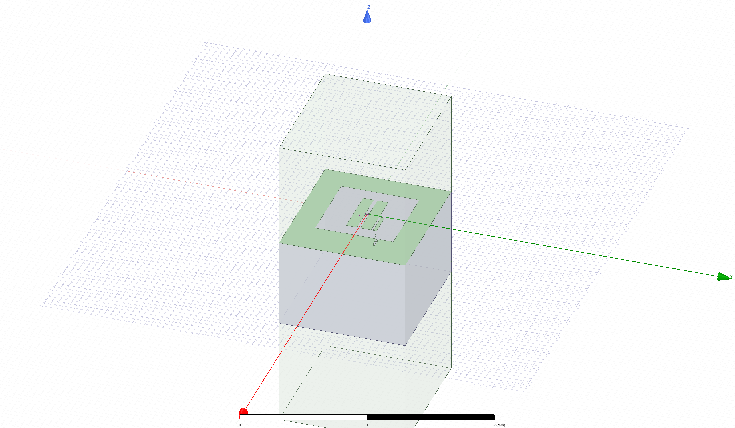
Render the single qubit in Metal, called Q1, to “TransmonQubit” design in Ansys.
[11]:
hfss.render_design(['Q1'], [])
hfss.save_screenshot()
Set the convergence parameters and junction properties in the Ansys design. Then run the analysis and plot the convergence.
[12]:
# Analysis properties
setup = hfss.pinfo.setup
setup.passes = 10
print(f"""
Number of eigenmodes to find             = {setup.n_modes}
Number of simulation passes              = {setup.passes}
Convergence freq max delta percent diff  = {setup.delta_f}
""")

pinfo = hfss.pinfo
pinfo.design.set_variable('Lj', '10 nH')
pinfo.design.set_variable('Cj', '0 fF')

setup.analyze()
INFO 09:14AM [analyze]: Analyzing setup Setup
Number of eigenmodes to find             = 1
Number of simulation passes              = 10
Convergence freq max delta percent diff  = 0.1
To plot the results you can use the plot_convergences() method from the eig_qb.sim object. The method will read the data from the variables local to the eig_qb.sim object, so we first need to assign the simulation results to these two variables. let’s do both (assignment and plotting) in the next cell.
[13]:
eig_qb.sim.convergence_t, eig_qb.sim.convergence_f, _ = hfss.get_convergences()
eig_qb.sim.plot_convergences()
09:15AM 39s INFO [get_f_convergence]: Saved convergences to C:\workspace\qiskit-metal\docs\tut\4-Analysis\hfss_eig_f_convergence.csv
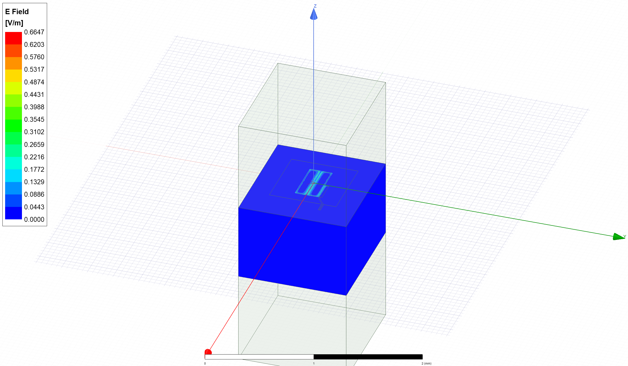
Display the Ansys modeler window and plot the E-field on the chip’s surface.
[14]:
hfss.modeler._modeler.ShowWindow()
hfss.plot_fields('main')
hfss.save_screenshot()
[14]:
WindowsPath('C:/workspace/qiskit-metal/docs/tut/4-Analysis/ansys.png')
Delete the newly created E-field plot to prepare for the next phase.
[15]:
hfss.plot_ansys_delete(['Mag_E1'])
09:15AM 44s WARNING [plot_ansys_delete]: This method is deprecated. Change your scripts to use clear_fields()
In the suggested (tutorial 4.2) flow, we would now prepare the setup using eig_qb.setup and run the analysis with eig_qb.run_epr(). Notice that this method requires previous set of the eig_qb variables convergence_t and convergence_f like we did a thee cells earlier.
However we here exemplify the advanced approach, which is Ansys-specific since it uses the pyEPR module methods directly. #### Setup Identify the non-linear (Josephson) junctions in the model. You will need to list the junctions in the epr setup.
In this case there’s only one junction, namely ‘jj’. Let’s see what we need to change in the default setup.
[16]:
pinfo = hfss.pinfo
pinfo.junctions['jj'] = {'Lj_variable': 'Lj', 'rect': 'JJ_rect_Lj_Q1_rect_jj',
                             'line': 'JJ_Lj_Q1_rect_jj_',  'Cj_variable': 'Cj'}
pinfo.validate_junction_info() # Check that valid names of variables and objects have been supplied
pinfo.dissipative['dielectrics_bulk'] = ['main'] # Dissipative elements: specify
Execute microwave analysis on eigenmode solutions.
[17]:
eprd = epr.DistributedAnalysis(pinfo)
Design "TransmonQubit" info:
        # eigenmodes    1
        # variations    1
Find the electric and magnetic energy stored in the substrate and the system as a whole.
[18]:
ℰ_elec = eprd.calc_energy_electric()
ℰ_elec_substrate = eprd.calc_energy_electric(None, 'main')
ℰ_mag = eprd.calc_energy_magnetic()

print(f"""
ℰ_elec_all       = {ℰ_elec}
ℰ_elec_substrate = {ℰ_elec_substrate}
EPR of substrate = {ℰ_elec_substrate / ℰ_elec * 100 :.1f}%

ℰ_mag    = {ℰ_mag}
""")
ℰ_elec_all       = 9.6815388026089e-25
ℰ_elec_substrate = 8.91706074244017e-25
EPR of substrate = 92.1%

ℰ_mag    = 2.44586411178151e-26
Perform EPR analysis for all modes and variations.
[19]:
eprd.do_EPR_analysis()

# 4a. Perform Hamiltonian spectrum post-analysis, building on mw solutions using EPR
epra = epr.QuantumAnalysis(eprd.data_filename)
epra.analyze_all_variations(cos_trunc = 8, fock_trunc = 7)

# 4b. Report solved results
swp_variable = 'Lj' # suppose we swept an optimetric analysis vs. inductance Lj_alice
epra.plot_hamiltonian_results(swp_variable=swp_variable)
epra.report_results(swp_variable=swp_variable, numeric=True)
Variation 0  [1/1]

  Mode 0 at 6.36 GHz   [1/1]
    Calculating ℰ_magnetic,ℰ_electric
       (ℰ_E-ℰ_H)/ℰ_E       ℰ_E       ℰ_H
               97.5%  4.841e-25 1.223e-26

    Calculating junction energy participation ration (EPR)
        method=`line_voltage`. First estimates:
        junction        EPR p_0j   sign s_0j    (p_capacitive)
                Energy fraction (Lj over Lj&Cj)= 96.90%
        jj              0.994495  (+)        0.0318047
                (U_tot_cap-U_tot_ind)/mean=0.59%
Calculating Qdielectric_main for mode 0 (0/0)
p_dielectric_main_0 = 0.9210375462253237
WARNING 09:15AM [__init__]: <p>Error: <class 'IndexError'></p>
ANALYSIS DONE. Data saved to:

C:\data-pyEPR\Project23\TransmonQubit\2021-07-20 09-15-44.npz


         Differences in variations:


 . . . . . . . . . . . . . . . . . . . . . . . . . . . . . . . . . . . . . . . .
Variation 0

Starting the diagonalization
Finished the diagonalization
Pm_norm=
modes
0    1.011964
dtype: float64

Pm_norm idx =
     jj
0  True
*** P (participation matrix, not normlz.)
         jj
0  0.963841

*** S (sign-bit matrix)
   s_jj
0     1
*** P (participation matrix, normalized.)
      0.98

*** Chi matrix O1 PT (MHz)
    Diag is anharmonicity, off diag is full cross-Kerr.
       295

*** Chi matrix ND (MHz)
       326

*** Frequencies O1 PT (MHz)
0    6069.617909
dtype: float64

*** Frequencies ND (MHz)
0    6054.749316
dtype: float64

*** Q_coupling
Empty DataFrame
Columns: []
Index: [0]
Mode frequencies (MHz)
Numerical diagonalization
| Lj | 10 |
|---|---|
| eigenmode | |
| 0 | 6069.62 |
Kerr Non-linear coefficient table (MHz)
Numerical diagonalization
| 0 | ||
|---|---|---|
| Lj | ||
| 10 | 0 | 325.92 |
Release Ansys session
[20]:
eig_qb.sim.close()
3. Analyze the transmon using the LOM method
In this section we will use a semi-manual (advanced) analysis flow. Please refer to tutorial 4.1 for the suggested method. As illustrated, the methods are equivalent, but the advanced method allows you to directly override some renderer-specific settings.
Select the analysis you intend to run from the qiskit_metal.analyses collection. Select the design to analyze and the tool to use for any external simulation.
[21]:
from qiskit_metal.analyses.quantization import LOManalysis
c1 = LOManalysis(design, "q3d")
For the capacitive simulation portion, you can either: 1. Use the c1 user-friendly methods (see tutorial 4.1) 2. Control directly the simulation tool from the tool’s GUI (outside metal - see specific vendor instructions) 3. Use the renderer methods In this section we show the advanced method (method 3).
The renderer can be reached from the analysis class. Let’s give it a shorter alias.
[22]:
q3d = c1.sim.renderer
Now we connect to the simulation tool, similarly to what we have done for the eigenmode analysis.
[23]:
q3d.start()
INFO 09:15AM [connect_project]: Connecting to Ansys Desktop API...
INFO 09:15AM [load_ansys_project]:      Opened Ansys App
INFO 09:15AM [load_ansys_project]:      Opened Ansys Desktop v2020.2.0
INFO 09:15AM [load_ansys_project]:      Opened Ansys Project
        Folder:    C:/Ansoft/
        Project:   Project23
INFO 09:15AM [connect_design]:  Opened active design
        Design:    TransmonQubit [Solution type: Eigenmode]
INFO 09:15AM [get_setup]:       Opened setup `Setup`  (<class 'pyEPR.ansys.HfssEMSetup'>)
INFO 09:15AM [connect]:         Connected to project "Project23" and design "TransmonQubit" 😀
[23]:
True
If the simulator is already open, the line above will simply connect to the open session, project and design.
Create and activate a q3d design called “TransmonQubit_q3d”.
[24]:
q3d.activate_ansys_design("TransmonQubit_q3d", 'capacitive') # use new_ansys_design() to force creation of a blank design
09:15AM 50s WARNING [activate_ansys_design]: The design_name=TransmonQubit_q3d was not in active project.  Designs in active project are:
['TransmonQubit'].  A new design will be added to the project.
INFO 09:15AM [connect_design]:  Opened active design
        Design:    TransmonQubit_q3d [Solution type: Q3D]
WARNING 09:15AM [connect_setup]:        No design setup detected.
WARNING 09:15AM [connect_setup]:        Creating Q3D default setup.
INFO 09:15AM [get_setup]:       Opened setup `Setup`  (<class 'pyEPR.ansys.AnsysQ3DSetup'>)
Next, we render the qubit to Ansys Q3D for analysis. We set the readout pin of the qubit in the ‘open’ termination list of the render so its capacitance is properly simulated.
[25]:
q3d.render_design(['Q1'], [('Q1','readout')])
Execute the capacitance extraction and verify converengence. This cell analyzes the default setup.
[26]:
q3d.analyze_setup("Setup")
INFO 09:15AM [get_setup]:       Opened setup `Setup`  (<class 'pyEPR.ansys.AnsysQ3DSetup'>)
INFO 09:15AM [analyze]: Analyzing setup Setup
This simulation had 4 nets, the two charge islands of the floating transmon, the readout coupler, and the ground, resulting in a 4x4 capacitance matrix. Output is of type DataFrame.
[27]:
c1.sim.capacitance_matrix, c1.sim.units = q3d.get_capacitance_matrix()
c1.sim.capacitance_all_passes, _ = q3d.get_capacitance_all_passes()
c1.sim.capacitance_matrix
INFO 09:16AM [get_matrix]: Exporting matrix data to (C:\Temp\tmpiarcjm5j.txt, C, , Setup:LastAdaptive, "Original", "ohm", "nH", "fF", "mSie", 5000000000, Maxwell, 1, False
INFO 09:16AM [get_matrix]: Exporting matrix data to (C:\Temp\tmpepo9v8c_.txt, C, , Setup:AdaptivePass, "Original", "ohm", "nH", "fF", "mSie", 5000000000, Maxwell, 1, False
INFO 09:16AM [get_matrix]: Exporting matrix data to (C:\Temp\tmpm0vz3x8k.txt, C, , Setup:AdaptivePass, "Original", "ohm", "nH", "fF", "mSie", 5000000000, Maxwell, 2, False
INFO 09:16AM [get_matrix]: Exporting matrix data to (C:\Temp\tmpzjrhgc8i.txt, C, , Setup:AdaptivePass, "Original", "ohm", "nH", "fF", "mSie", 5000000000, Maxwell, 3, False
INFO 09:16AM [get_matrix]: Exporting matrix data to (C:\Temp\tmpl1y179u_.txt, C, , Setup:AdaptivePass, "Original", "ohm", "nH", "fF", "mSie", 5000000000, Maxwell, 4, False
INFO 09:16AM [get_matrix]: Exporting matrix data to (C:\Temp\tmpdkn79c7o.txt, C, , Setup:AdaptivePass, "Original", "ohm", "nH", "fF", "mSie", 5000000000, Maxwell, 5, False
INFO 09:16AM [get_matrix]: Exporting matrix data to (C:\Temp\tmpm2ju65p3.txt, C, , Setup:AdaptivePass, "Original", "ohm", "nH", "fF", "mSie", 5000000000, Maxwell, 6, False
INFO 09:16AM [get_matrix]: Exporting matrix data to (C:\Temp\tmpnsg_76lo.txt, C, , Setup:AdaptivePass, "Original", "ohm", "nH", "fF", "mSie", 5000000000, Maxwell, 7, False
INFO 09:16AM [get_matrix]: Exporting matrix data to (C:\Temp\tmpx6ny8pav.txt, C, , Setup:AdaptivePass, "Original", "ohm", "nH", "fF", "mSie", 5000000000, Maxwell, 8, False
INFO 09:16AM [get_matrix]: Exporting matrix data to (C:\Temp\tmp24_r0zj2.txt, C, , Setup:AdaptivePass, "Original", "ohm", "nH", "fF", "mSie", 5000000000, Maxwell, 9, False
INFO 09:16AM [get_matrix]: Exporting matrix data to (C:\Temp\tmpzhx0_ygi.txt, C, , Setup:AdaptivePass, "Original", "ohm", "nH", "fF", "mSie", 5000000000, Maxwell, 10, False
[27]:
| ground_main_plane | pad_bot_Q1 | pad_top_Q1 | readout_connector_pad_Q1 | |
|---|---|---|---|---|
| ground_main_plane | 177.78538 | -44.74611 | -38.34722 | -37.03041 |
| pad_bot_Q1 | -44.74611 | 82.84141 | -32.48515 | -2.30760 |
| pad_top_Q1 | -38.34722 | -32.48515 | 93.38943 | -19.67329 |
| readout_connector_pad_Q1 | -37.03041 | -2.30760 | -19.67329 | 60.14998 |
Now we provide the junction lumped element values, and complete the analysis by plotting the convergence. This is the same steps used in the suggested flow from tutorial 4.1.
[28]:
c1.setup.junctions=Dict(Lj=12.31, Cj=2)
c1.setup.freq_readout = 7.0
c1.setup.freq_bus = []

c1.run_lom()
c1.lumped_oscillator_all
[1, 2] [3]
Predicted Values

Transmon Properties
f_Q 5.492369 [GHz]
EC 320.340887 [MHz]
EJ 13.273404 [GHz]
alpha -374.552102 [MHz]
dispersion 58.767574 [KHz]
Lq 12.305036 [nH]
Cq 60.467548 [fF]
T1 47.110126 [us]

**Coupling Properties**

tCqbus1 -7.535751 [fF]
gbus1_in_MHz -119.111599 [MHz]
χ_bus1 -3.815566 [MHz]
1/T1bus1 3378.359561 [Hz]
T1bus1 47.110126 [us]
Bus-Bus Couplings
[28]:
| fQ | EC | EJ | alpha | dispersion | gbus | chi_in_MHz | χr MHz | gr MHz | |
|---|---|---|---|---|---|---|---|---|---|
| 1 | 5.848645 | 366.675723 | 13.273404 | -435.120535 | 183.838223 | [-120.91915969031888] | [-7.045838787793941] | 7.045839 | 120.919160 |
| 2 | 5.800484 | 360.198673 | 13.273404 | -426.554207 | 158.894188 | [-112.57027192270645] | [-5.610759520303708] | 5.610760 | 112.570272 |
| 3 | 5.728978 | 350.706154 | 13.273404 | -414.05886 | 127.373567 | [-114.4721344200509] | [-5.135837723457538] | 5.135838 | 114.472134 |
| 4 | 5.645726 | 339.839946 | 13.273404 | -399.840701 | 97.757395 | [-113.75236108111946] | [-4.422671613573481] | 4.422672 | 113.752361 |
| 5 | 5.574615 | 330.715418 | 13.273404 | -387.971176 | 77.483483 | [-115.42485160814473] | [-4.067027529550902] | 4.067028 | 115.424852 |
| 6 | 5.552051 | 327.850119 | 13.273404 | -384.256913 | 71.883362 | [-116.90656488361248] | [-4.027920633490058] | 4.027921 | 116.906565 |
| 7 | 5.522295 | 324.093652 | 13.273404 | -379.396816 | 65.050231 | [-118.53068129631139] | [-3.9548493935622147] | 3.954849 | 118.530681 |
| 8 | 5.508895 | 322.410099 | 13.273404 | -377.222089 | 62.166575 | [-118.93049750280109] | [-3.9007913880708722] | 3.900791 | 118.930498 |
| 9 | 5.492369 | 320.340887 | 13.273404 | -374.552102 | 58.767574 | [-119.11159900747404] | [-3.8155660691691082] | 3.815566 | 119.111599 |
And plot the convergence.
[29]:
c1.plot_convergence();
c1.plot_convergence_chi()
Design "TransmonQubit_q3d" info:
        # eigenmodes    0
        # variations    1
INFO 09:16AM [hfss_report_full_convergence]: Creating report for variation 0
Release the simulator and close the analysis.
[30]:
c1.sim.close()
(optional) close the GUI.
[31]:
# gui.main_window.close()
For more information, review the Introduction to Quantum Computing and Quantum Hardware lectures below
|
Lecture Video | Lecture Notes | Lab |
|
Lecture Video | Lecture Notes | Lab |
|
Lecture Video | Lecture Notes | Lab |
|
Lecture Video | Lecture Notes | Lab |
|
Lecture Video | Lecture Notes | Lab |
|
Lecture Video | Lecture Notes | Lab |