注釈
このページは docs/tutorials/10_qgan_option_pricing.ipynb から生成されました。
qGANs によるオプション価格推定#
はじめに#
このnotebookでは、量子機械学習アルゴリズムについて説明します。 すなわち、量子敵対的生成ネットワーク(qGAN)は、ヨーロピアン・コール・オプションの価格設定を容易にすることができます。 具体的には、量子回路がヨーロピアン・コール・オプションの基盤となる資産のスポット価格をモデル化するように、qGANを訓練することができます。 得られたモデルを量子振幅推定に基づくアルゴリズムに統合して、期待されるペイオフを評価することができます。 ヨーロピアン・コール・オプションの価格推 を参照してください。qGANの学習によるランダム分布の学習とロードの詳細については、次の文献を参照してください。 Quantum Generative Adversarial Networks for Learning and Loading Random Distributions. Zoufal, Lucchi, Woerner. 2019.
[1]:
import matplotlib.pyplot as plt
import numpy as np

from qiskit.circuit import ParameterVector
from qiskit.circuit.library import TwoLocal
from qiskit.quantum_info import Statevector

from qiskit_algorithms import IterativeAmplitudeEstimation, EstimationProblem
from qiskit_aer.primitives import Sampler
from qiskit_finance.applications.estimation import EuropeanCallPricing
from qiskit_finance.circuit.library import NormalDistribution
不確実性モデル#
Black-Scholes モデルでは、ヨーロピアン・コール・オプションの満期の \(S_T\) のスポット価格が対数正規分布であると仮定しています。 よって、対数正規分布からのサンプルでqGANを訓練し、結果をオプションの背後にある不確実性モデルとして使用することができます。 以下では、不確実性モデルをロードする量子回路を構築し、回路出力が読み込まれます。
ここで、\(j\in \left\{0, \ldots, {2^n-1} \right\}\) における確率 \(p_{\theta}^{j}\) はターゲット分布のモデルを表します。
[2]:
# Set upper and lower data values
bounds = np.array([0.0, 7.0])
# Set number of qubits used in the uncertainty model
num_qubits = 3

# Load the trained circuit parameters
g_params = [0.29399714, 0.38853322, 0.9557694, 0.07245791, 6.02626428, 0.13537225]

# Set an initial state for the generator circuit
init_dist = NormalDistribution(num_qubits, mu=1.0, sigma=1.0, bounds=bounds)

# construct the variational form
var_form = TwoLocal(num_qubits, "ry", "cz", entanglement="circular", reps=1)

# keep a list of the parameters so we can associate them to the list of numerical values
# (otherwise we need a dictionary)
theta = var_form.ordered_parameters

# compose the generator circuit, this is the circuit loading the uncertainty model
g_circuit = init_dist.compose(var_form)
期待ペイオフの評価#
これで、訓練された不確実性モデルは、オプションのペイオフ関数の期待値を分析的に、そして量子振幅推定を用いて評価するために使用できるようになりました。
[3]:
# set the strike price (should be within the low and the high value of the uncertainty)
strike_price = 2

# set the approximation scaling for the payoff function
c_approx = 0.25
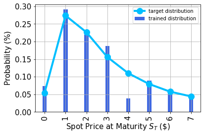
確率分布をプロットする#
次に、訓練された確率分布と、比較のために目標の確率分布をプロットします。
[4]:
# Evaluate trained probability distribution
values = [
    bounds[0] + (bounds[1] - bounds[0]) * x / (2**num_qubits - 1) for x in range(2**num_qubits)
]
uncertainty_model = g_circuit.assign_parameters(dict(zip(theta, g_params)))
amplitudes = Statevector.from_instruction(uncertainty_model).data

x = np.array(values)
y = np.abs(amplitudes) ** 2

# Sample from target probability distribution
N = 100000
log_normal = np.random.lognormal(mean=1, sigma=1, size=N)
log_normal = np.round(log_normal)
log_normal = log_normal[log_normal <= 7]
log_normal_samples = []
for i in range(8):
    log_normal_samples += [np.sum(log_normal == i)]
log_normal_samples = np.array(log_normal_samples / sum(log_normal_samples))

# Plot distributions
plt.bar(x, y, width=0.2, label="trained distribution", color="royalblue")
plt.xticks(x, size=15, rotation=90)
plt.yticks(size=15)
plt.grid()
plt.xlabel("Spot Price at Maturity $S_T$ (\$)", size=15)
plt.ylabel("Probability ($\%$)", size=15)
plt.plot(
    log_normal_samples,
    "-o",
    color="deepskyblue",
    label="target distribution",
    linewidth=4,
    markersize=12,
)
plt.legend(loc="best")
plt.show()
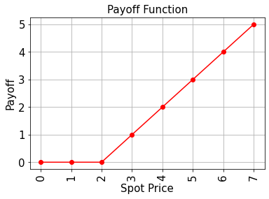
期待ペイオフの評価#
これにより、訓練された不確実性モデルを使用して、量子振幅推定を用いたオプションのペイオフ関数の期待値を分析できるようになりました。
[5]:
# Evaluate payoff for different distributions
payoff = np.array([0, 0, 0, 1, 2, 3, 4, 5])
ep = np.dot(log_normal_samples, payoff)
print("Analytically calculated expected payoff w.r.t. the target distribution:  %.4f" % ep)
ep_trained = np.dot(y, payoff)
print("Analytically calculated expected payoff w.r.t. the trained distribution: %.4f" % ep_trained)

# Plot exact payoff function (evaluated on the grid of the trained uncertainty model)
x = np.array(values)
y_strike = np.maximum(0, x - strike_price)
plt.plot(x, y_strike, "ro-")
plt.grid()
plt.title("Payoff Function", size=15)
plt.xlabel("Spot Price", size=15)
plt.ylabel("Payoff", size=15)
plt.xticks(x, size=15, rotation=90)
plt.yticks(size=15)
plt.show()
Analytically calculated expected payoff w.r.t. the target distribution:  1.0611
Analytically calculated expected payoff w.r.t. the trained distribution: 0.9805
[6]:
# construct circuit for payoff function
european_call_pricing = EuropeanCallPricing(
    num_qubits,
    strike_price=strike_price,
    rescaling_factor=c_approx,
    bounds=bounds,
    uncertainty_model=uncertainty_model,
)
[7]:
# set target precision and confidence level
epsilon = 0.01
alpha = 0.05

problem = european_call_pricing.to_estimation_problem()
# construct amplitude estimation
ae = IterativeAmplitudeEstimation(
    epsilon_target=epsilon, alpha=alpha, sampler=Sampler(run_options={"shots": 100, "seed": 75})
)
[8]:
result = ae.estimate(problem)
[9]:
conf_int = np.array(result.confidence_interval_processed)
print("Exact value:        \t%.4f" % ep_trained)
print("Estimated value:    \t%.4f" % (result.estimation_processed))
print("Confidence interval:\t[%.4f, %.4f]" % tuple(conf_int))
Exact value:            0.9805
Estimated value:        1.0138
Confidence interval:    [0.9883, 1.0394]
[10]:
import qiskit.tools.jupyter

%qiskit_version_table
%qiskit_copyright
Version Information
| Software | Version |
|---|---|
qiskit | None |
qiskit-terra | 0.45.0.dev0+c626be7 |
qiskit_algorithms | 0.2.0 |
qiskit_aer | 0.12.0 |
qiskit_optimization | 0.6.0 |
qiskit_finance | 0.4.0 |
qiskit_ibm_provider | 0.6.1 |
| System information | |
| Python version | 3.9.7 |
| Python compiler | GCC 7.5.0 |
| Python build | default, Sep 16 2021 13:09:58 |
| OS | Linux |
| CPUs | 2 |
| Memory (Gb) | 5.778430938720703 |
| Fri Aug 18 16:26:01 2023 EDT | |
This code is a part of Qiskit
© Copyright IBM 2017, 2023.
This code is licensed under the Apache License, Version 2.0. You may
obtain a copy of this license in the LICENSE.txt file in the root directory
of this source tree or at http://www.apache.org/licenses/LICENSE-2.0.
Any modifications or derivative works of this code must retain this
copyright notice, and modified files need to carry a notice indicating
that they have been altered from the originals.
[ ]: