注釈
このページは docs/tutorials/08_fixed_income_pricing.ipynb から生成されました。
固定収入資産の価格推定#
はじめに#
我々は金利の確率分布が分かっている固定収入資産の価格推定をします。資産のキャッシュフロー \(c_t\) とキャッシュフローの期日は既知とします。資産の合計価値 \(V\) は次の期待値になります:
各キャッシュフローは、満期日に依存する、金利 \(r_t\) のゼロ・クーポン債として扱われます。ユーザーは各 \(r_t\) の(相関する可能性がある)不確実性モデルの確率分布と、サンプルに使う量子ビット数を指定しなければなりません。この例では我々は資産価値を金利 \(r_t\) の一次関数で展開します。これは資産を期間の観点で調査することにあたります。目的関数の近似は次の論文に従います: Quantum Risk Analysis. Woerner, Egger. 2018.
[1]:
import matplotlib.pyplot as plt

%matplotlib inline
import numpy as np
from qiskit import QuantumCircuit
from qiskit_algorithms import IterativeAmplitudeEstimation, EstimationProblem
from qiskit_aer.primitives import Sampler
from qiskit_finance.circuit.library import NormalDistribution
不確実性モデル#
\(d\) 次元多変量正規分布を量子状態にロードする回路を構築します。その分布は所与のボックス \(\otimes_{i=1}^d [low_i, high_i]\) に切り詰め、 \(2^{n_i}\) グリッドに離散化します。ここで \(n_i\) は、 \(i = 1,\ldots, d\) 次元で使用される量子ビット数です。この回路のユニタリー演算子は次のようになります:
ここで \(p_{i_1, ..., i_d}\) は、切り捨てられ離散化された分布を与える確率を表し、 \(i_j\) はアフィン写像で得られた正しい区間 \([low_j, high_j]\) です。
不確実性モデルに加えて、我々はアフィン写像を適用することもできます。例えば、主成分分析などが挙げられます。使用される金利は以下で与えられます。
ここで \(\vec{x} \in \otimes_{i=1}^d [low_i, high_i]\) は与えられた確率分布に従います。
[2]:
# can be used in case a principal component analysis has been done to derive the uncertainty model, ignored in this example.
A = np.eye(2)
b = np.zeros(2)

# specify the number of qubits that are used to represent the different dimenions of the uncertainty model
num_qubits = [2, 2]

# specify the lower and upper bounds for the different dimension
low = [0, 0]
high = [0.12, 0.24]
mu = [0.12, 0.24]
sigma = 0.01 * np.eye(2)

# construct corresponding distribution
bounds = list(zip(low, high))
u = NormalDistribution(num_qubits, mu, sigma, bounds)
[3]:
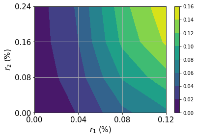
# plot contour of probability density function
x = np.linspace(low[0], high[0], 2 ** num_qubits[0])
y = np.linspace(low[1], high[1], 2 ** num_qubits[1])
z = u.probabilities.reshape(2 ** num_qubits[0], 2 ** num_qubits[1])
plt.contourf(x, y, z)
plt.xticks(x, size=15)
plt.yticks(y, size=15)
plt.grid()
plt.xlabel("$r_1$ (%)", size=15)
plt.ylabel("$r_2$ (%)", size=15)
plt.colorbar()
plt.show()
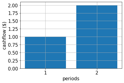
キャッシュフロー、ペイオフ関数、そして正確な期待値#
以下では、期間あたりのキャッシュフロー、結果として得られるペイオフ関数を定義し、正確な期待値を評価します。
ペイオフ関数は、最初に一次近似を使用しますが、その後 ヨーロピアン・コール・オプション のペイオフ関数の線形部分と同じ近似テクニックを適用します。
[4]:
# specify cash flow
cf = [1.0, 2.0]
periods = range(1, len(cf) + 1)

# plot cash flow
plt.bar(periods, cf)
plt.xticks(periods, size=15)
plt.yticks(size=15)
plt.grid()
plt.xlabel("periods", size=15)
plt.ylabel("cashflow ($)", size=15)
plt.show()
[5]:
# estimate real value
cnt = 0
exact_value = 0.0
for x1 in np.linspace(low[0], high[0], pow(2, num_qubits[0])):
    for x2 in np.linspace(low[1], high[1], pow(2, num_qubits[1])):
        prob = u.probabilities[cnt]
        for t in range(len(cf)):
            # evaluate linear approximation of real value w.r.t. interest rates
            exact_value += prob * (
                cf[t] / pow(1 + b[t], t + 1)
                - (t + 1) * cf[t] * np.dot(A[:, t], np.asarray([x1, x2])) / pow(1 + b[t], t + 2)
            )
        cnt += 1
print("Exact value:    \t%.4f" % exact_value)
Exact value: 2.1942
[6]:
# specify approximation factor
c_approx = 0.125

# create fixed income pricing application
from qiskit_finance.applications.estimation import FixedIncomePricing

fixed_income = FixedIncomePricing(
    num_qubits=num_qubits,
    pca_matrix=A,
    initial_interests=b,
    cash_flow=cf,
    rescaling_factor=c_approx,
    bounds=bounds,
    uncertainty_model=u,
)
[7]:
fixed_income._objective.draw()
[7]:
     ┌────┐
q_0: ┤0   ├
     │    │
q_1: ┤1   ├
     │    │
q_2: ┤2 F ├
     │    │
q_3: ┤3   ├
     │    │
q_4: ┤4   ├
     └────┘
[8]:
fixed_income_circ = QuantumCircuit(fixed_income._objective.num_qubits)

# load probability distribution
fixed_income_circ.append(u, range(u.num_qubits))

# apply function
fixed_income_circ.append(fixed_income._objective, range(fixed_income._objective.num_qubits))

fixed_income_circ.draw()
[8]:
     ┌───────┐┌────┐
q_0: ┤0      ├┤0   ├
     │       ││    │
q_1: ┤1      ├┤1   ├
     │  P(X) ││    │
q_2: ┤2      ├┤2 F ├
     │       ││    │
q_3: ┤3      ├┤3   ├
     └───────┘│    │
q_4: ─────────┤4   ├
              └────┘
[9]:
# set target precision and confidence level
epsilon = 0.01
alpha = 0.05

# construct amplitude estimation
problem = fixed_income.to_estimation_problem()

ae = IterativeAmplitudeEstimation(
    epsilon_target=epsilon, alpha=alpha, sampler=Sampler(run_options={"shots": 100, "seed": 75})
)
[10]:
result = ae.estimate(problem)
[11]:
conf_int = np.array(result.confidence_interval_processed)
print("Exact value:        \t%.4f" % exact_value)
print("Estimated value:    \t%.4f" % (fixed_income.interpret(result)))
print("Confidence interval:\t[%.4f, %.4f]" % tuple(conf_int))
Exact value:            2.1942
Estimated value:        2.3437
Confidence interval:    [2.3101, 2.3772]
[12]:
import qiskit.tools.jupyter

%qiskit_version_table
%qiskit_copyright
Version Information
| Software | Version |
|---|---|
qiskit | None |
qiskit-terra | 0.45.0.dev0+c626be7 |
qiskit_finance | 0.4.0 |
qiskit_algorithms | 0.2.0 |
qiskit_ibm_provider | 0.6.1 |
qiskit_optimization | 0.6.0 |
qiskit_aer | 0.12.0 |
| System information | |
| Python version | 3.9.7 |
| Python compiler | GCC 7.5.0 |
| Python build | default, Sep 16 2021 13:09:58 |
| OS | Linux |
| CPUs | 2 |
| Memory (Gb) | 5.778430938720703 |
| Fri Aug 18 16:21:18 2023 EDT | |
This code is a part of Qiskit
© Copyright IBM 2017, 2023.
This code is licensed under the Apache License, Version 2.0. You may
obtain a copy of this license in the LICENSE.txt file in the root directory
of this source tree or at http://www.apache.org/licenses/LICENSE-2.0.
Any modifications or derivative works of this code must retain this
copyright notice, and modified files need to carry a notice indicating
that they have been altered from the originals.
[ ]: