注釈
このページは docs/tutorials/07_asian_barrier_spread_pricing.ipynb から生成されました。
アジアン・バリア・スプレッドの価格推定#
はじめに#
アジアン・バリア・スプレッドは3つの異なるタイプを組み合わせたオプションで、それゆえに Qiskit Finance オプションの価格設定フレームワークがサポートする複数の機能を組み合わせています。
アジアン・オプション: ペイオフが対象期間の平均価格によって変化します。
バリア・オプション: ペイオフが対象期間中に閾値を超えるとゼロになります。
(ブル)・スプレッド: ペイオフはゼロから始まり、線形に増加し、一定に維持される、(平均価格に依存した) 区分線形関数に従います。
権利行使価格 \(K_1 < K_2\) と期間 \(t=1,2\) が,与えられた多変量分布(確率過程によって生成されたものなど)に従うスポット価格 \((S_1, S_2)\) とバリアしきい値 \(B>0\) に対応するとします。対応するペイオフ関数は次のように定義されます。
以下では、振幅推定に基づく量子アルゴリズムを使用して、期待されるペイオフ、すなわちオプションの割引前の適正価格を見積もります。
目的関数の近似と量子コンピューターによる一般的なオプション価格設定とリスク分析は、以下の論文で紹介されています。
[1]:
import matplotlib.pyplot as plt
from scipy.interpolate import griddata

%matplotlib inline
import numpy as np

from qiskit import QuantumRegister, QuantumCircuit, AncillaRegister, transpile
from qiskit.circuit.library import IntegerComparator, WeightedAdder, LinearAmplitudeFunction
from qiskit_algorithms import IterativeAmplitudeEstimation, EstimationProblem
from qiskit_aer.primitives import Sampler
from qiskit_finance.circuit.library import LogNormalDistribution
不確実性モデル#
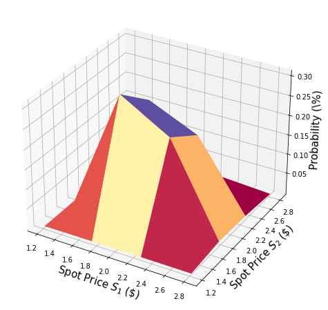
多変量対数正規ランダム分布を \(n\) 量子ビットの量子状態にロードする回路を構築します。 すべての次元 \(j = 1,\ldots,d\) について、分布は指定された区間 \([\text{low}_j, \text{high}_j]\) に切り捨てられ、 \(2^{n_j}\) グリッドポイントを使用して離散化されます。ここで、 \(n_j\) は次元 \(j\) を表すために使用される量子ビットの数を示します。つまり \(n_1+\ldots+n_d = n\) です。 回路に対応するユニタリー演算子は、以下のように実装されます:
ここで \(p_{i_1\ldots i_d}\) は、切り捨てられ離散化された分布を与える確率を表し、 \(i_j\) はアフィン写像で正しい区間にマップされます。
簡単のため、株価はどちらも独立同分布とします。この仮定は以下のパラメーター化を単純にするだけのものであり、より複雑で相関のある多変量分布に容易に緩和することができます。現在の実装で唯一の重要な仮定は、異なる次元の離散化グリッドが同じステップサイズであるということです。
[2]:
# number of qubits per dimension to represent the uncertainty
num_uncertainty_qubits = 2

# parameters for considered random distribution
S = 2.0  # initial spot price
vol = 0.4  # volatility of 40%
r = 0.05  # annual interest rate of 4%
T = 40 / 365  # 40 days to maturity

# resulting parameters for log-normal distribution
mu = (r - 0.5 * vol**2) * T + np.log(S)
sigma = vol * np.sqrt(T)
mean = np.exp(mu + sigma**2 / 2)
variance = (np.exp(sigma**2) - 1) * np.exp(2 * mu + sigma**2)
stddev = np.sqrt(variance)

# lowest and highest value considered for the spot price; in between, an equidistant discretization is considered.
low = np.maximum(0, mean - 3 * stddev)
high = mean + 3 * stddev

# map to higher dimensional distribution
# for simplicity assuming dimensions are independent and identically distributed)
dimension = 2
num_qubits = [num_uncertainty_qubits] * dimension
low = low * np.ones(dimension)
high = high * np.ones(dimension)
mu = mu * np.ones(dimension)
cov = sigma**2 * np.eye(dimension)

# construct circuit
u = LogNormalDistribution(num_qubits=num_qubits, mu=mu, sigma=cov, bounds=(list(zip(low, high))))
[3]:
# plot PDF of uncertainty model
x = [v[0] for v in u.values]
y = [v[1] for v in u.values]
z = u.probabilities
# z = map(float, z)
# z = list(map(float, z))
resolution = np.array([2**n for n in num_qubits]) * 1j
grid_x, grid_y = np.mgrid[min(x) : max(x) : resolution[0], min(y) : max(y) : resolution[1]]
grid_z = griddata((x, y), z, (grid_x, grid_y))
plt.figure(figsize=(10, 8))
ax = plt.axes(projection="3d")
ax.plot_surface(grid_x, grid_y, grid_z, cmap=plt.cm.Spectral)
ax.set_xlabel("Spot Price $S_1$ (\$)", size=15)
ax.set_ylabel("Spot Price $S_2$ (\$)", size=15)
ax.set_zlabel("Probability (\%)", size=15)
plt.show()
ペイオフ関数#
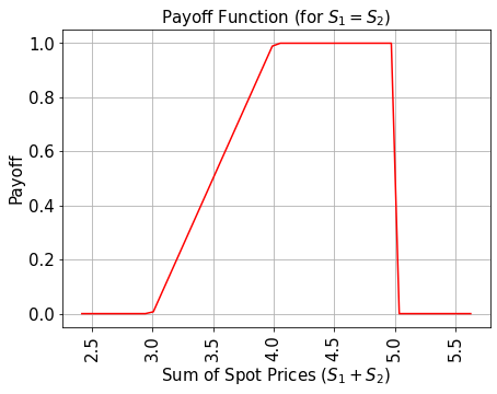
簡単のため、平均の代わりにスポット価格の合計を考えます。結果を2で割るだけで平均にできます。
ペイオフ関数は、スポット価格合計 \((S_1 + S_2)\) が権利行使価格 \(K_1\) よりも小さい間ゼロであり、その後スポット価格合計が \(K_2\) になるまで線形に増加します。そしてペイオフはどちらかのスポット価格がバリアしきい値 \(B\) を超えるまで、一定 \(K_2 - K_1\) ですが、その後ペイオフは直ちにゼロに落ちます。実装では初め加重合計演算子を使って補助量子ビットにスポット価格合計を計算しますが、それからコンパレーターを使って、もし \((S_1 + S_2) \geq K_1\) ならば補助量子ビットを \(\big|0\rangle\) to \(\big|1\rangle\) にフリップします。そしてもう一つのコンパレーターと補助量子ビットを \((S_1 + S_2) \geq K_2\) のケースを記録するためにフリップします。これらの補助量子ビットはペイオフ関数の線形部分をコントロールするために使われます。
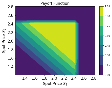
それに加え、別の補助量子ビットを時間ステップごとに追加します。そして追加のコンパレーターで \(S_1\) とそれぞれの \(S_2\) がバリアしきい値 \(B\) を超えていないかチェックします。ペイオフ関数は \(S_1, S_2 \leq B\) の場合のみ適用されます。
線形部分自体は次のように近似されます。 小さい \(|y|\) に対して \(\sin^2(y + \pi/4) \approx y + 1/2\) という事実を利用します。 したがって、与えられた近似スケーリング係数 \(c_\text{approx} \in [0, 1]\) および \(x \in [0, 1]\) に対して、次を考えます。
ここで、\(c_\text{approx}\) は十分小さいものとします。
次のように機能する演算子を簡単に構築できます
制御 Y-回転を用います。
最終的には、 \(\sin^2(a*x+b)\) に対応する最後の量子ビットで \(\big|1\rangle\) を測定する確率に関心があります。 上記の近似と合わせて、対象の値を近似できます。小さい \(c_\text{approx}\) を選択するほど、近似は良くなります。 ただし、 \(c_\text{approx}\) でスケーリングされたプロパティを推定しているため、それに応じて評価量子ビットの数 \(m\) を調整する必要があります。
近似の詳細については、次を参照してください: Quantum Risk Analysis. Woerner, Egger. 2018.
(現在実装中の) 加重合計演算子は整数のみを合計することができるため、結果を推定するために元の範囲から表現可能な範囲に写像し、結果を解釈する前に逆写像する必要があります。このマッピングは不確定性モデルのコンテキストに出てきたアフィン写像に一致します。
[4]:
# determine number of qubits required to represent total loss
weights = []
for n in num_qubits:
    for i in range(n):
        weights += [2**i]

# create aggregation circuit
agg = WeightedAdder(sum(num_qubits), weights)
n_s = agg.num_sum_qubits
n_aux = agg.num_qubits - n_s - agg.num_state_qubits  # number of additional qubits
[5]:
# set the strike price (should be within the low and the high value of the uncertainty)
strike_price_1 = 3
strike_price_2 = 4

# set the barrier threshold
barrier = 2.5

# map strike prices and barrier threshold from [low, high] to {0, ..., 2^n-1}
max_value = 2**n_s - 1
low_ = low[0]
high_ = high[0]

mapped_strike_price_1 = (
    (strike_price_1 - dimension * low_) / (high_ - low_) * (2**num_uncertainty_qubits - 1)
)
mapped_strike_price_2 = (
    (strike_price_2 - dimension * low_) / (high_ - low_) * (2**num_uncertainty_qubits - 1)
)
mapped_barrier = (barrier - low) / (high - low) * (2**num_uncertainty_qubits - 1)
[6]:
# condition and condition result
conditions = []
barrier_thresholds = [2] * dimension
n_aux_conditions = 0
for i in range(dimension):
    # target dimension of random distribution and corresponding condition (which is required to be True)
    comparator = IntegerComparator(num_qubits[i], mapped_barrier[i] + 1, geq=False)
    n_aux_conditions = max(n_aux_conditions, comparator.num_ancillas)
    conditions += [comparator]
[7]:
# set the approximation scaling for the payoff function
c_approx = 0.25

# setup piecewise linear objective fcuntion
breakpoints = [0, mapped_strike_price_1, mapped_strike_price_2]
slopes = [0, 1, 0]
offsets = [0, 0, mapped_strike_price_2 - mapped_strike_price_1]
f_min = 0
f_max = mapped_strike_price_2 - mapped_strike_price_1
objective = LinearAmplitudeFunction(
    n_s,
    slopes,
    offsets,
    domain=(0, max_value),
    image=(f_min, f_max),
    rescaling_factor=c_approx,
    breakpoints=breakpoints,
)
[8]:
# define overall multivariate problem
qr_state = QuantumRegister(u.num_qubits, "state")  # to load the probability distribution
qr_obj = QuantumRegister(1, "obj")  # to encode the function values
ar_sum = AncillaRegister(n_s, "sum")  # number of qubits used to encode the sum
ar_cond = AncillaRegister(len(conditions) + 1, "conditions")
ar = AncillaRegister(
    max(n_aux, n_aux_conditions, objective.num_ancillas), "work"
)  # additional qubits

objective_index = u.num_qubits

# define the circuit
asian_barrier_spread = QuantumCircuit(qr_state, qr_obj, ar_cond, ar_sum, ar)

# load the probability distribution
asian_barrier_spread.append(u, qr_state)

# apply the conditions
for i, cond in enumerate(conditions):
    state_qubits = qr_state[(num_uncertainty_qubits * i) : (num_uncertainty_qubits * (i + 1))]
    asian_barrier_spread.append(cond, state_qubits + [ar_cond[i]] + ar[: cond.num_ancillas])

# aggregate the conditions on a single qubit
asian_barrier_spread.mcx(ar_cond[:-1], ar_cond[-1])

# apply the aggregation function controlled on the condition
asian_barrier_spread.append(agg.control(), [ar_cond[-1]] + qr_state[:] + ar_sum[:] + ar[:n_aux])

# apply the payoff function
asian_barrier_spread.append(objective, ar_sum[:] + qr_obj[:] + ar[: objective.num_ancillas])

# uncompute the aggregation
asian_barrier_spread.append(
    agg.inverse().control(), [ar_cond[-1]] + qr_state[:] + ar_sum[:] + ar[:n_aux]
)

# uncompute the conditions
asian_barrier_spread.mcx(ar_cond[:-1], ar_cond[-1])

for j, cond in enumerate(reversed(conditions)):
    i = len(conditions) - j - 1
    state_qubits = qr_state[(num_uncertainty_qubits * i) : (num_uncertainty_qubits * (i + 1))]
    asian_barrier_spread.append(
        cond.inverse(), state_qubits + [ar_cond[i]] + ar[: cond.num_ancillas]
    )

print(asian_barrier_spread.draw())
print("objective qubit index", objective_index)
              ┌───────┐┌──────┐             ┌───────────┐      ┌──────────────┐»
     state_0: ┤0      ├┤0     ├─────────────┤1          ├──────┤1             ├»
              │       ││      │             │           │      │              │»
     state_1: ┤1      ├┤1     ├─────────────┤2          ├──────┤2             ├»
              │  P(X) ││      │┌──────┐     │           │      │              │»
     state_2: ┤2      ├┤      ├┤0     ├─────┤3          ├──────┤3             ├»
              │       ││      ││      │     │           │      │              │»
     state_3: ┤3      ├┤      ├┤1     ├─────┤4          ├──────┤4             ├»
              └───────┘│      ││      │     │           │┌────┐│              │»
         obj: ─────────┤      ├┤      ├─────┤           ├┤3   ├┤              ├»
                       │      ││      │     │           ││    ││              │»
conditions_0: ─────────┤2     ├┤      ├──■──┤           ├┤    ├┤              ├»
                       │  cmp ││      │  │  │           ││    ││              │»
conditions_1: ─────────┤      ├┤2     ├──■──┤           ├┤    ├┤              ├»
                       │      ││  cmp │┌─┴─┐│   c_adder ││    ││   c_adder_dg │»
conditions_2: ─────────┤      ├┤      ├┤ X ├┤0          ├┤    ├┤0             ├»
                       │      ││      │└───┘│           ││    ││              │»
       sum_0: ─────────┤      ├┤      ├─────┤5          ├┤0   ├┤5             ├»
                       │      ││      │     │           ││  F ││              │»
       sum_1: ─────────┤      ├┤      ├─────┤6          ├┤1   ├┤6             ├»
                       │      ││      │     │           ││    ││              │»
       sum_2: ─────────┤      ├┤      ├─────┤7          ├┤2   ├┤7             ├»
                       │      ││      │     │           ││    ││              │»
      work_0: ─────────┤3     ├┤3     ├─────┤8          ├┤4   ├┤8             ├»
                       └──────┘└──────┘     │           ││    ││              │»
      work_1: ──────────────────────────────┤9          ├┤5   ├┤9             ├»
                                            │           ││    ││              │»
      work_2: ──────────────────────────────┤10         ├┤6   ├┤10            ├»
                                            └───────────┘└────┘└──────────────┘»
«                              ┌─────────┐
«     state_0: ────────────────┤0        ├
«                              │         │
«     state_1: ────────────────┤1        ├
«                   ┌─────────┐│         │
«     state_2: ─────┤0        ├┤         ├
«                   │         ││         │
«     state_3: ─────┤1        ├┤         ├
«                   │         ││         │
«         obj: ─────┤         ├┤         ├
«                   │         ││         │
«conditions_0: ──■──┤         ├┤2        ├
«                │  │         ││  cmp_dg │
«conditions_1: ──■──┤2        ├┤         ├
«              ┌─┴─┐│  cmp_dg ││         │
«conditions_2: ┤ X ├┤         ├┤         ├
«              └───┘│         ││         │
«       sum_0: ─────┤         ├┤         ├
«                   │         ││         │
«       sum_1: ─────┤         ├┤         ├
«                   │         ││         │
«       sum_2: ─────┤         ├┤         ├
«                   │         ││         │
«      work_0: ─────┤3        ├┤3        ├
«                   └─────────┘└─────────┘
«      work_1: ───────────────────────────
«
«      work_2: ───────────────────────────
«
objective qubit index 4
[9]:
# plot exact payoff function
plt.figure(figsize=(7, 5))
x = np.linspace(sum(low), sum(high))
y = (x <= 5) * np.minimum(np.maximum(0, x - strike_price_1), strike_price_2 - strike_price_1)
plt.plot(x, y, "r-")
plt.grid()
plt.title("Payoff Function (for $S_1 = S_2$)", size=15)
plt.xlabel("Sum of Spot Prices ($S_1 + S_2)$", size=15)
plt.ylabel("Payoff", size=15)
plt.xticks(size=15, rotation=90)
plt.yticks(size=15)
plt.show()
[10]:
# plot contour of payoff function with respect to both time steps, including barrier
plt.figure(figsize=(7, 5))
z = np.zeros((17, 17))
x = np.linspace(low[0], high[0], 17)
y = np.linspace(low[1], high[1], 17)
for i, x_ in enumerate(x):
    for j, y_ in enumerate(y):
        z[i, j] = np.minimum(
            np.maximum(0, x_ + y_ - strike_price_1), strike_price_2 - strike_price_1
        )
        if x_ > barrier or y_ > barrier:
            z[i, j] = 0

plt.title("Payoff Function", size=15)
plt.contourf(x, y, z)
plt.colorbar()
plt.xlabel("Spot Price $S_1$", size=15)
plt.ylabel("Spot Price $S_2$", size=15)
plt.xticks(size=15)
plt.yticks(size=15)
plt.show()
[11]:
# evaluate exact expected value
sum_values = np.sum(u.values, axis=1)
payoff = np.minimum(np.maximum(sum_values - strike_price_1, 0), strike_price_2 - strike_price_1)
leq_barrier = [np.max(v) <= barrier for v in u.values]
exact_value = np.dot(u.probabilities[leq_barrier], payoff[leq_barrier])
print("exact expected value:\t%.4f" % exact_value)
exact expected value: 0.8023
期待ペイオフの評価#
我々は、まず量子回路を検証します。シミュレートで目的量子ビットの \(|1\rangle\) 状態の観測確率を分析します。
[12]:
num_state_qubits = asian_barrier_spread.num_qubits - asian_barrier_spread.num_ancillas
print("state qubits: ", num_state_qubits)
transpiled = transpile(asian_barrier_spread, basis_gates=["u", "cx"])
print("circuit width:", transpiled.width())
print("circuit depth:", transpiled.depth())
state qubits:  5
circuit width: 14
circuit depth: 6373
[13]:
asian_barrier_spread_measure = asian_barrier_spread.measure_all(inplace=False)
sampler = Sampler()
job = sampler.run(asian_barrier_spread_measure)
[14]:
# evaluate the result
value = 0
probabilities = job.result().quasi_dists[0].binary_probabilities()
for i, prob in probabilities.items():
    if prob > 1e-4 and i[-num_state_qubits:][0] == "1":
        value += prob


# map value to original range
mapped_value = objective.post_processing(value) / (2**num_uncertainty_qubits - 1) * (high_ - low_)
print("Exact Operator Value:  %.4f" % value)
print("Mapped Operator value: %.4f" % mapped_value)
print("Exact Expected Payoff: %.4f" % exact_value)
Exact Operator Value:  0.6455
Mapped Operator value: 0.8705
Exact Expected Payoff: 0.8023
次に振幅推定で期待ペイオフを推定します。多数の量子ビットをシミュレートするため、推定には時間がかかることに注意してください。我々が設計した演算子 (asian_barrier_spread) は実際の状態量子ビット数よりもかなり少なくなっていますが、これはシミュレーション時間を短縮するためです。
[15]:
# set target precision and confidence level
epsilon = 0.01
alpha = 0.05

problem = EstimationProblem(
    state_preparation=asian_barrier_spread,
    objective_qubits=[objective_index],
    post_processing=objective.post_processing,
)
# construct amplitude estimation
ae = IterativeAmplitudeEstimation(
    epsilon, alpha=alpha, sampler=Sampler(run_options={"shots": 100, "seed": 75})
)
[16]:
result = ae.estimate(problem)
[17]:
conf_int = (
    np.array(result.confidence_interval_processed)
    / (2**num_uncertainty_qubits - 1)
    * (high_ - low_)
)
print("Exact value:    \t%.4f" % exact_value)
print(
    "Estimated value:\t%.4f"
    % (result.estimation_processed / (2**num_uncertainty_qubits - 1) * (high_ - low_))
)
print("Confidence interval: \t[%.4f, %.4f]" % tuple(conf_int))
Exact value:            0.8023
Estimated value:        0.8320
Confidence interval:    [0.8264, 0.8376]
[18]:
import qiskit.tools.jupyter

%qiskit_version_table
%qiskit_copyright
Version Information
| Software | Version |
|---|---|
qiskit | None |
qiskit-terra | 0.45.0.dev0+c626be7 |
qiskit_aer | 0.12.0 |
qiskit_ibm_provider | 0.6.1 |
qiskit_algorithms | 0.2.0 |
qiskit_finance | 0.4.0 |
| System information | |
| Python version | 3.9.7 |
| Python compiler | GCC 7.5.0 |
| Python build | default, Sep 16 2021 13:09:58 |
| OS | Linux |
| CPUs | 2 |
| Memory (Gb) | 5.778430938720703 |
| Fri Aug 18 16:20:04 2023 EDT | |
This code is a part of Qiskit
© Copyright IBM 2017, 2023.
This code is licensed under the Apache License, Version 2.0. You may
obtain a copy of this license in the LICENSE.txt file in the root directory
of this source tree or at http://www.apache.org/licenses/LICENSE-2.0.
Any modifications or derivative works of this code must retain this
copyright notice, and modified files need to carry a notice indicating
that they have been altered from the originals.
[ ]: