注釈
このページは docs/tutorials/03_european_call_option_pricing.ipynb から生成されました。
ヨーロピアン・コール・オプションの価格推定#
はじめに#
権利行使価格 \(K\) で、原資産の満期時のスポット価格 \(S_T\) がある確率分布に従うヨーロピアン・コール・オプションを考えます。 その時のペイオフ関数は次のように定義されます:
以下では、振幅推定に基づく量子アルゴリズムを使用して、期待されるペイオフ、すなわちオプションの割引前の適正価格を見積もります。
同様に対応する \(\Delta\)、すなわちスポット価格に対するオプション価格の微分係数は、次のように与えられます:
目的関数の近似と量子コンピューターによる一般的なオプション価格設定とリスク分析は、以下の論文で紹介されています。
[1]:
import matplotlib.pyplot as plt

%matplotlib inline
import numpy as np

from qiskit import QuantumCircuit
from qiskit_algorithms import IterativeAmplitudeEstimation, EstimationProblem
from qiskit.circuit.library import LinearAmplitudeFunction
from qiskit_aer.primitives import Sampler
from qiskit_finance.circuit.library import LogNormalDistribution
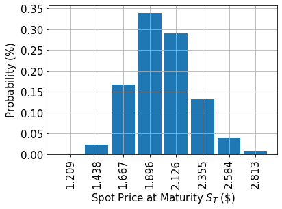
不確実性モデル#
対数正規分布を量子状態にロードする回路を構築します。 分布は \([\text{low}, \text{high}]\) で指定された区間に切り捨てられ、 \(2^n\) グリッドに離散化されます。ここで \(n\) は使用する量子ビット数です。この回路に対応するユニタリー演算子は、次のように実装されます:
ここで \(p_i\) は切り捨てられ離散化された分布を与える確率を表し、\(i\) はアフィン写像で得られた正しい区間です。
[2]:
# number of qubits to represent the uncertainty
num_uncertainty_qubits = 3

# parameters for considered random distribution
S = 2.0  # initial spot price
vol = 0.4  # volatility of 40%
r = 0.05  # annual interest rate of 4%
T = 40 / 365  # 40 days to maturity

# resulting parameters for log-normal distribution
mu = (r - 0.5 * vol**2) * T + np.log(S)
sigma = vol * np.sqrt(T)
mean = np.exp(mu + sigma**2 / 2)
variance = (np.exp(sigma**2) - 1) * np.exp(2 * mu + sigma**2)
stddev = np.sqrt(variance)

# lowest and highest value considered for the spot price; in between, an equidistant discretization is considered.
low = np.maximum(0, mean - 3 * stddev)
high = mean + 3 * stddev

# construct A operator for QAE for the payoff function by
# composing the uncertainty model and the objective
uncertainty_model = LogNormalDistribution(
    num_uncertainty_qubits, mu=mu, sigma=sigma**2, bounds=(low, high)
)
[3]:
# plot probability distribution
x = uncertainty_model.values
y = uncertainty_model.probabilities
plt.bar(x, y, width=0.2)
plt.xticks(x, size=15, rotation=90)
plt.yticks(size=15)
plt.grid()
plt.xlabel("Spot Price at Maturity $S_T$ (\$)", size=15)
plt.ylabel("Probability ($\%$)", size=15)
plt.show()
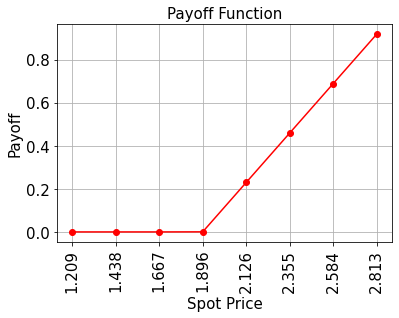
ペイオフ関数#
ペイオフ関数は、満期時のスポット価格 \(S_T\) が権利行使価格 \(K\) よりも小さい間はゼロであり、その後、線形に増加します。実装はコンパレーターを使用し、もし \(S_T \geq K\) ならば補助量子ビットを \(\big|0\rangle\) から \(\big|1\rangle\) にフリップし、この補助量子ビットがペイオフ関数の線形部分を制御します。
線形部分自体は、次のように近似されます。 小さい \(|y|\) に対して \(\sin^2(y + \pi/4) \approx y + 1/2\) という事実を利用します。 したがって、与えられた近似再スケーリング係数 \(c_\text{approx} \in [0, 1]\) および \(x \in [0, 1]\) に対して、以下を考えます。
ここで、\(c_\text{approx}\) は十分小さいものとします。
次のように機能する演算子を簡単に構築できます
制御Y-回転を使います。
最終的には、 \(\sin^2(a*x+b)\) に対応する最後の量子ビットで \(\big|1\rangle\) を測定する確率に関心があります。 上記の近似と合わせて、対象の値を近似できます。小さい \(c_\text{approx}\) を選択するほど、近似は良くなります。 ただし、 \(c_\text{approx}\) でスケーリングされたプロパティを推定しているため、それに応じて評価量子ビットの数 \(m\) を調整する必要があります。
近似の詳細については、次を参照してください: Quantum Risk Analysis. Woerner, Egger. 2018.
[4]:
# set the strike price (should be within the low and the high value of the uncertainty)
strike_price = 1.896

# set the approximation scaling for the payoff function
c_approx = 0.25

# setup piecewise linear objective fcuntion
breakpoints = [low, strike_price]
slopes = [0, 1]
offsets = [0, 0]
f_min = 0
f_max = high - strike_price
european_call_objective = LinearAmplitudeFunction(
    num_uncertainty_qubits,
    slopes,
    offsets,
    domain=(low, high),
    image=(f_min, f_max),
    breakpoints=breakpoints,
    rescaling_factor=c_approx,
)

# construct A operator for QAE for the payoff function by
# composing the uncertainty model and the objective
num_qubits = european_call_objective.num_qubits
european_call = QuantumCircuit(num_qubits)
european_call.append(uncertainty_model, range(num_uncertainty_qubits))
european_call.append(european_call_objective, range(num_qubits))

# draw the circuit
european_call.draw()
[4]:
     ┌───────┐┌────┐
q_0: ┤0      ├┤0   ├
     │       ││    │
q_1: ┤1 P(X) ├┤1   ├
     │       ││    │
q_2: ┤2      ├┤2   ├
     └───────┘│    │
q_3: ─────────┤3 F ├
              │    │
q_4: ─────────┤4   ├
              │    │
q_5: ─────────┤5   ├
              │    │
q_6: ─────────┤6   ├
              └────┘
[5]:
# plot exact payoff function (evaluated on the grid of the uncertainty model)
x = uncertainty_model.values
y = np.maximum(0, x - strike_price)
plt.plot(x, y, "ro-")
plt.grid()
plt.title("Payoff Function", size=15)
plt.xlabel("Spot Price", size=15)
plt.ylabel("Payoff", size=15)
plt.xticks(x, size=15, rotation=90)
plt.yticks(size=15)
plt.show()
[6]:
# evaluate exact expected value (normalized to the [0, 1] interval)
exact_value = np.dot(uncertainty_model.probabilities, y)
exact_delta = sum(uncertainty_model.probabilities[x >= strike_price])
print("exact expected value:\t%.4f" % exact_value)
print("exact delta value:   \t%.4f" % exact_delta)
exact expected value:   0.1623
exact delta value:      0.8098
期待ペイオフの評価#
[7]:
european_call.draw()
[7]:
     ┌───────┐┌────┐
q_0: ┤0      ├┤0   ├
     │       ││    │
q_1: ┤1 P(X) ├┤1   ├
     │       ││    │
q_2: ┤2      ├┤2   ├
     └───────┘│    │
q_3: ─────────┤3 F ├
              │    │
q_4: ─────────┤4   ├
              │    │
q_5: ─────────┤5   ├
              │    │
q_6: ─────────┤6   ├
              └────┘
[8]:
# set target precision and confidence level
epsilon = 0.01
alpha = 0.05

problem = EstimationProblem(
    state_preparation=european_call,
    objective_qubits=[3],
    post_processing=european_call_objective.post_processing,
)
# construct amplitude estimation
ae = IterativeAmplitudeEstimation(
    epsilon_target=epsilon, alpha=alpha, sampler=Sampler(run_options={"shots": 100, "seed": 75})
)
[9]:
result = ae.estimate(problem)
[10]:
conf_int = np.array(result.confidence_interval_processed)
print("Exact value:        \t%.4f" % exact_value)
print("Estimated value:    \t%.4f" % (result.estimation_processed))
print("Confidence interval:\t[%.4f, %.4f]" % tuple(conf_int))
Exact value:            0.1623
Estimated value:        0.1687
Confidence interval:    [0.1637, 0.1737]
これらの回路を手動で構築する代わりに、Qiskit Finance モジュールは EuropeanCallPricing 回路を提供しています。この回路は、この機能をビルディングブロックとしてすでに実装しています。
[11]:
from qiskit_finance.applications.estimation import EuropeanCallPricing

european_call_pricing = EuropeanCallPricing(
    num_state_qubits=num_uncertainty_qubits,
    strike_price=strike_price,
    rescaling_factor=c_approx,
    bounds=(low, high),
    uncertainty_model=uncertainty_model,
)
[12]:
# set target precision and confidence level
epsilon = 0.01
alpha = 0.05

problem = european_call_pricing.to_estimation_problem()
# construct amplitude estimation
ae = IterativeAmplitudeEstimation(
    epsilon_target=epsilon, alpha=alpha, sampler=Sampler(run_options={"shots": 100, "seed": 75})
)
result = ae.estimate(problem)

conf_int = np.array(result.confidence_interval_processed)
print("Exact value:        \t%.4f" % exact_value)
print("Estimated value:    \t%.4f" % (european_call_pricing.interpret(result)))
print("Confidence interval:\t[%.4f, %.4f]" % tuple(conf_int))
Exact value:            0.1623
Estimated value:        0.1687
Confidence interval:    [0.1637, 0.1737]
デルタの評価#
デルタは期待ペイオフよりも少し評価が簡単です。 期待ペイオフと同様に、コンパレータ回路と補助量子ビットを使用して、 \(S_T > K\) の場合を特定します。しかしながら、この条件が真であるときの確率のみに興味があるので、振幅推定において他に何も仮定せずにこの補助量子ビットを直接目的量子ビットとして使うことができます。
[13]:
from qiskit_finance.applications.estimation import EuropeanCallDelta

european_call_delta = EuropeanCallDelta(
    num_state_qubits=num_uncertainty_qubits,
    strike_price=strike_price,
    bounds=(low, high),
    uncertainty_model=uncertainty_model,
)
[14]:
european_call_delta._objective.decompose().draw()
[14]:
         ┌──────┐
state_0: ┤0     ├
         │      │
state_1: ┤1     ├
         │      │
state_2: ┤2     ├
         │  cmp │
state_3: ┤3     ├
         │      │
 work_0: ┤4     ├
         │      │
 work_1: ┤5     ├
         └──────┘
[15]:
european_call_delta_circ = QuantumCircuit(european_call_delta._objective.num_qubits)
european_call_delta_circ.append(uncertainty_model, range(num_uncertainty_qubits))
european_call_delta_circ.append(
    european_call_delta._objective, range(european_call_delta._objective.num_qubits)
)

european_call_delta_circ.draw()
[15]:
     ┌───────┐┌──────┐
q_0: ┤0      ├┤0     ├
     │       ││      │
q_1: ┤1 P(X) ├┤1     ├
     │       ││      │
q_2: ┤2      ├┤2     ├
     └───────┘│  ECD │
q_3: ─────────┤3     ├
              │      │
q_4: ─────────┤4     ├
              │      │
q_5: ─────────┤5     ├
              └──────┘
[16]:
# set target precision and confidence level
epsilon = 0.01
alpha = 0.05

problem = european_call_delta.to_estimation_problem()

# construct amplitude estimation
ae_delta = IterativeAmplitudeEstimation(
    epsilon_target=epsilon, alpha=alpha, sampler=Sampler(run_options={"shots": 100, "seed": 75})
)
[17]:
result_delta = ae_delta.estimate(problem)
[18]:
conf_int = np.array(result_delta.confidence_interval_processed)
print("Exact delta:    \t%.4f" % exact_delta)
print("Estimated value: \t%.4f" % european_call_delta.interpret(result_delta))
print("Confidence interval: \t[%.4f, %.4f]" % tuple(conf_int))
Exact delta:            0.8098
Estimated value:        0.8091
Confidence interval:    [0.8034, 0.8148]
[19]:
import qiskit.tools.jupyter

%qiskit_version_table
%qiskit_copyright
Version Information
| Software | Version |
|---|---|
qiskit | None |
qiskit-terra | 0.45.0.dev0+c626be7 |
qiskit_finance | 0.4.0 |
qiskit_aer | 0.12.0 |
qiskit_algorithms | 0.2.0 |
qiskit_ibm_provider | 0.6.1 |
qiskit_optimization | 0.6.0 |
| System information | |
| Python version | 3.9.7 |
| Python compiler | GCC 7.5.0 |
| Python build | default, Sep 16 2021 13:09:58 |
| OS | Linux |
| CPUs | 2 |
| Memory (Gb) | 5.778430938720703 |
| Fri Aug 18 16:00:58 2023 EDT | |
This code is a part of Qiskit
© Copyright IBM 2017, 2023.
This code is licensed under the Apache License, Version 2.0. You may
obtain a copy of this license in the LICENSE.txt file in the root directory
of this source tree or at http://www.apache.org/licenses/LICENSE-2.0.
Any modifications or derivative works of this code must retain this
copyright notice, and modified files need to carry a notice indicating
that they have been altered from the originals.
[ ]: