注釈

このページは docs/tutorials/09_credit_risk_analysis.ipynb から生成されました。

信用リスク分析#

はじめに#

このチュートリアルは、どのように量子アルゴリズムが信用リスク分析に使えるかを示します。より正確には、どのように量子振幅推定(QAE) が古典的なモンテカルロシミュレーションに比べて二次のスピードアップでリスク推定ができるかを示します。このチュートリアルは次の論文に基づいています:

Quantum Risk Analysis. Stefan Woerner, Daniel J. Egger. [Woerner2019]
Credit Risk Analysis using Quantum Computers. Egger et al. (2019) [Egger2019]

QAE の一般的な紹介は、次の論文にあります:

Quantum Amplitude Amplification and Estimation. Gilles Brassard et al.

このチュートリアルの構造は、次のとおりです：

問題定義
不確実性モデル
期待損失
累積分布関数
バリュー・アット・リスク
条件付きバリュー・アット・リスク

[1]:

import numpy as np
import matplotlib.pyplot as plt

from qiskit import QuantumRegister, QuantumCircuit
from qiskit.circuit.library import IntegerComparator
from qiskit_algorithms import IterativeAmplitudeEstimation, EstimationProblem
from qiskit_aer.primitives import Sampler

問題定義#

このチュートリアルでは \(K\) 個の資産からなるポートフォリオの信用リスクを分析します。それぞれの資産 \(k\) のデフォルト確率は ガウス型条件付き独立 モデルに従います。すなわち、標準正規分布に従う潜在乱数 \(Z\) からサンプルされた値 \(z\) が与えられると、資産 \(k\) のデフォルト確率は次で与えられます。

\[p_k(z) = F\left( \frac{F^{-1}(p_k^0) - \sqrt{\rho_k}z}{\sqrt{1 - \rho_k}} \right)\]

ここで \(F\) は \(Z\) の累積確率分布、 \(p_k^0\) は資産 \(k\) の \(z=0\) におけるデフォルト確率、そして \(\rho_k\) は資産 \(k\) の \(Z\) におけるデフォルト確率の感度です。こうして \(Z\) の具体形が与えられ、個別のデフォルトイベントはそれぞれ独立とみなされます。

我々は総損失のリスク分析に興味があります。

\[L = \sum_{k=1}^K \lambda_k X_k(Z)\]

ここで \(\lambda_k\) は資産 \(k\) の デフォルトによる損失 を意味し、\(Z\) 、 \(X_k(Z)\) は資産 \(k\) のデフォルトイベントに対するベルヌーイ変数です。より正確に、我々は期待値 \(\mathbb{E}[L]\) 、\(L\) のバリュー・アット・リスク(VaR)と \(L\) の条件付きバリュー・アット・リスク(期待ショートフォールとも呼ばれる)に興味があります。ここで VaR と CVaR は次のように定義されます。

\[\text{VaR}_{\alpha}(L) = \inf \{ x \mid \mathbb{P}[L <= x] \geq 1 - \alpha \}\]

信頼レベル \(\alpha \in [0, 1]\), および

\[\text{CVaR}_{\alpha}(L) = \mathbb{E}[ L \mid L \geq \text{VaR}_{\alpha}(L) ].\]

検討されたモデルの詳細については、例えば次の文献を参照してください Regulatory Capital Modeling for Credit Risk. Marek Rutkowski, Silvio Tarca

問題は以下のパラメータで定義されています:

\(Z\) を表現する量子ビット数、\(n_z\) で示されます。
\(Z\) の打切り値。\(z_{\text{max}}\) で表示されます。すなわち、Z は等間隔の値 \(\{-z_{max}, ..., +z_{max}\}\) の \(2^{n_z}\) をとるとみなされます。
各資産のベースデフォルト確率。\(p_0^k \in (0, 1)\), \(k=1, ..., K\)
\(Z\) に関するデフォルト確率の敏感性。\(\rho_k \in [0, 1)\) で表示されます。
資産 \(k\) のデフォルト時損失率。 \(\lambda_k\) で表示されます。
VaR / CVaR の信頼水準 \(\alpha \in [0, 1]\)。

[2]:

# set problem parameters
n_z = 2
z_max = 2
z_values = np.linspace(-z_max, z_max, 2**n_z)
p_zeros = [0.15, 0.25]
rhos = [0.1, 0.05]
lgd = [1, 2]
K = len(p_zeros)
alpha = 0.05

不確実性モデル#

我々は不確実性モデルをロードする回路を構築します。これは標準正規分布に従う \(Z\) を表現する \(n_z\) 個の量子ビットの量子状態を作ることで達成されます。この状態は、\(K\) ビットの２つ目の量子レジスター上で、単一量子ビットの Y 回転を制御するために使われます。ここで量子ビット \(k\) の \(|1\rangle\) 状態は資産 \(k\) のデフォルトイベントを表します。その結果、量子状態は次のように記述できます

\[ |\Psi\rangle = \sum_{i=0}^{2^{n_z}-1} \sqrt{p_z^i} |z_i \rangle \bigotimes_{k=1}^K \left( \sqrt{1 - p_k(z_i)}|0\rangle + \sqrt{p_k(z_i)}|1\rangle\right),\]

ここで \(z_i\) は、切り捨てられ丸められた \(Z\) の \(i\) 番目の値を表します。[Egger2019].

[3]:

from qiskit_finance.circuit.library import GaussianConditionalIndependenceModel as GCI

u = GCI(n_z, z_max, p_zeros, rhos)

[4]:

u.draw()

[4]:

     ┌───────┐
q_0: ┤0      ├
     │       │
q_1: ┤1      ├
     │  P(X) │
q_2: ┤2      ├
     │       │
q_3: ┤3      ├
     └───────┘

ここで \(|\Psi\rangle\) を構成する回路を検証するためシミュレータを使用します。そして以下の関連する厳密値を計算します。

期待損失 \(\mathbb{E}[L]\)
\(L\) の PDF と CDF
バリューアットリスク \(VaR(L)\) と関連する確率
条件付きバリューアットリスク \(CVaR(L)\)

[5]:

u_measure = u.measure_all(inplace=False)
sampler = Sampler()
job = sampler.run(u_measure)
binary_probabilities = job.result().quasi_dists[0].binary_probabilities()

[6]:

# analyze uncertainty circuit and determine exact solutions
p_z = np.zeros(2**n_z)
p_default = np.zeros(K)
values = []
probabilities = []
num_qubits = u.num_qubits

for i, prob in binary_probabilities.items():
    # extract value of Z and corresponding probability
    i_normal = int(i[-n_z:], 2)
    p_z[i_normal] += prob

    # determine overall default probability for k
    loss = 0
    for k in range(K):
        if i[K - k - 1] == "1":
            p_default[k] += prob
            loss += lgd[k]

    values += [loss]
    probabilities += [prob]


values = np.array(values)
probabilities = np.array(probabilities)

expected_loss = np.dot(values, probabilities)
losses = np.sort(np.unique(values))
pdf = np.zeros(len(losses))
for i, v in enumerate(losses):
    pdf[i] += sum(probabilities[values == v])
cdf = np.cumsum(pdf)

i_var = np.argmax(cdf >= 1 - alpha)
exact_var = losses[i_var]
exact_cvar = np.dot(pdf[(i_var + 1) :], losses[(i_var + 1) :]) / sum(pdf[(i_var + 1) :])

[7]:

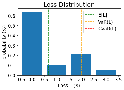
print("Expected Loss E[L]:                %.4f" % expected_loss)
print("Value at Risk VaR[L]:              %.4f" % exact_var)
print("P[L <= VaR[L]]:                    %.4f" % cdf[exact_var])
print("Conditional Value at Risk CVaR[L]: %.4f" % exact_cvar)

Expected Loss E[L]:                0.6641
Value at Risk VaR[L]:              2.0000
P[L <= VaR[L]]:                    0.9521
Conditional Value at Risk CVaR[L]: 3.0000

[8]:

# plot loss PDF, expected loss, var, and cvar
plt.bar(losses, pdf)
plt.axvline(expected_loss, color="green", linestyle="--", label="E[L]")
plt.axvline(exact_var, color="orange", linestyle="--", label="VaR(L)")
plt.axvline(exact_cvar, color="red", linestyle="--", label="CVaR(L)")
plt.legend(fontsize=15)
plt.xlabel("Loss L ($)", size=15)
plt.ylabel("probability (%)", size=15)
plt.title("Loss Distribution", size=20)
plt.xticks(size=15)
plt.yticks(size=15)
plt.show()

../_images/tutorials_09_credit_risk_analysis_12_0.png

[9]:

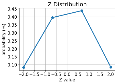
# plot results for Z
plt.plot(z_values, p_z, "o-", linewidth=3, markersize=8)
plt.grid()
plt.xlabel("Z value", size=15)
plt.ylabel("probability (%)", size=15)
plt.title("Z Distribution", size=20)
plt.xticks(size=15)
plt.yticks(size=15)
plt.show()

../_images/tutorials_09_credit_risk_analysis_13_0.png

[10]:

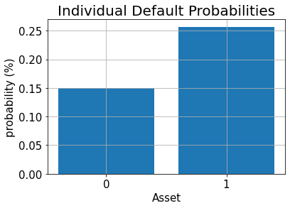
# plot results for default probabilities
plt.bar(range(K), p_default)
plt.xlabel("Asset", size=15)
plt.ylabel("probability (%)", size=15)
plt.title("Individual Default Probabilities", size=20)
plt.xticks(range(K), size=15)
plt.yticks(size=15)
plt.grid()
plt.show()

../_images/tutorials_09_credit_risk_analysis_14_0.png

期待損失#

期待損失を見積もるために、我々はまずはじめに加重合計演算子を適用し、個別損失を合計損失に足し上げます:

\[\mathcal{S}: |x_1, ..., x_K \rangle_K |0\rangle_{n_S} \mapsto |x_1, ..., x_K \rangle_K |\lambda_1x_1 + ... + \lambda_K x_K\rangle_{n_S}.\]

結果を表すために必要な量子ビット数は

\[n_s = \lfloor \log_2( \lambda_1 + ... + \lambda_K ) \rfloor + 1.\]

合計損失分布を量子レジスターに得られれば、[Woerner2019] に記述されたテクニックを使うことができます。次の演算子で合計損失 \(L \in \{0, ..., 2^{n_s}-1\}\) を目的量子ビットの振幅にマップします。

\[ | L \rangle_{n_s}|0\rangle \mapsto | L \rangle_{n_s} \left( \sqrt{1 - L/(2^{n_s}-1)}|0\rangle + \sqrt{L/(2^{n_s}-1)}|1\rangle \right),\]

これにより、期待損失を評価するために振幅推定を実行できます。

[11]:

# add Z qubits with weight/loss 0
from qiskit.circuit.library import WeightedAdder

agg = WeightedAdder(n_z + K, [0] * n_z + lgd)

[12]:

from qiskit.circuit.library import LinearAmplitudeFunction

# define linear objective function
breakpoints = [0]
slopes = [1]
offsets = [0]
f_min = 0
f_max = sum(lgd)
c_approx = 0.25

objective = LinearAmplitudeFunction(
    agg.num_sum_qubits,
    slope=slopes,
    offset=offsets,
    # max value that can be reached by the qubit register (will not always be reached)
    domain=(0, 2**agg.num_sum_qubits - 1),
    image=(f_min, f_max),
    rescaling_factor=c_approx,
    breakpoints=breakpoints,
)

状態準備回路を作成します:

[13]:

# define the registers for convenience and readability
qr_state = QuantumRegister(u.num_qubits, "state")
qr_sum = QuantumRegister(agg.num_sum_qubits, "sum")
qr_carry = QuantumRegister(agg.num_carry_qubits, "carry")
qr_obj = QuantumRegister(1, "objective")

# define the circuit
state_preparation = QuantumCircuit(qr_state, qr_obj, qr_sum, qr_carry, name="A")

# load the random variable
state_preparation.append(u.to_gate(), qr_state)

# aggregate
state_preparation.append(agg.to_gate(), qr_state[:] + qr_sum[:] + qr_carry[:])

# linear objective function
state_preparation.append(objective.to_gate(), qr_sum[:] + qr_obj[:])

# uncompute aggregation
state_preparation.append(agg.to_gate().inverse(), qr_state[:] + qr_sum[:] + qr_carry[:])

# draw the circuit
state_preparation.draw()

[13]:

           ┌───────┐┌────────┐      ┌───────────┐
  state_0: ┤0      ├┤0       ├──────┤0          ├
           │       ││        │      │           │
  state_1: ┤1      ├┤1       ├──────┤1          ├
           │  P(X) ││        │      │           │
  state_2: ┤2      ├┤2       ├──────┤2          ├
           │       ││        │      │           │
  state_3: ┤3      ├┤3       ├──────┤3          ├
           └───────┘│  adder │┌────┐│  adder_dg │
objective: ─────────┤        ├┤2   ├┤           ├
                    │        ││    ││           │
    sum_0: ─────────┤4       ├┤0 F ├┤4          ├
                    │        ││    ││           │
    sum_1: ─────────┤5       ├┤1   ├┤5          ├
                    │        │└────┘│           │
    carry: ─────────┤6       ├──────┤6          ├
                    └────────┘      └───────────┘

期待損失を見積もるために QAE を実行する前に、我々は目的関数の量子回路を直接シミュレートで検証し、目的量子ビットが \(|1\rangle\) 状態にいる確率を分析します。つまり、QAE の値は最終的に近似されます。

[14]:

state_preparation_measure = state_preparation.measure_all(inplace=False)
sampler = Sampler()
job = sampler.run(state_preparation_measure)
binary_probabilities = job.result().quasi_dists[0].binary_probabilities()

[15]:

# evaluate the result
value = 0
for i, prob in binary_probabilities.items():
    if prob > 1e-6 and i[-(len(qr_state) + 1) :][0] == "1":
        value += prob

print("Exact Expected Loss:   %.4f" % expected_loss)
print("Exact Operator Value:  %.4f" % value)
print("Mapped Operator value: %.4f" % objective.post_processing(value))

Exact Expected Loss:   0.6641
Exact Operator Value:  0.3789
Mapped Operator value: 0.5749

次に期待損失を推定するために、古典的モンテカルロ法よりも二次でスピードアップする QAE を実行します。

[16]:

# set target precision and confidence level
epsilon = 0.01
alpha = 0.05

problem = EstimationProblem(
    state_preparation=state_preparation,
    objective_qubits=[len(qr_state)],
    post_processing=objective.post_processing,
)
# construct amplitude estimation
ae = IterativeAmplitudeEstimation(
    epsilon_target=epsilon, alpha=alpha, sampler=Sampler(run_options={"shots": 100, "seed": 75})
)
result = ae.estimate(problem)

# print results
conf_int = np.array(result.confidence_interval_processed)
print("Exact value:    \t%.4f" % expected_loss)
print("Estimated value:\t%.4f" % result.estimation_processed)
print("Confidence interval: \t[%.4f, %.4f]" % tuple(conf_int))

Exact value:            0.6641
Estimated value:        0.6863
Confidence interval:    [0.6175, 0.7552]

累積分布関数#

(古典的な方法で効率的に推定できる) 期待損失の代わりに、損失の累積分布関数(CDF) を推定します。古典的には、資産デフォルトのすべての可能な組み合わせを評価するか、モンテカルロシミュレーションで多数の古典的サンプルを評価するか、どちらかを伴います。QAE に基づくアルゴリズムは将来大幅に解析をスピードアップする可能性があります。

CDF つまり確率 \(\mathbb{P}[L \leq x]\) を推定するために、再び \(\mathcal{S}\) を合計損失を計算するために適用し、そして与えられた \(x\) に対し以下のように振る舞うコンパレーターを適用します。

\[\begin{split} \mathcal{C}: |L\rangle_n|0> \mapsto \begin{cases} |L\rangle_n|1> & \text{if}\quad L \leq x \\ |L\rangle_n|0> & \text{if}\quad L > x. \end{cases}\end{split}\]

結果の量子状態は次のように記述でき、

\[ \sum_{L = 0}^{x} \sqrt{p_{L}}|L\rangle_{n_s}|1\rangle + \sum_{L = x+1}^{2^{n_s}-1} \sqrt{p_{L}}|L\rangle_{n_s}|0\rangle,\]

不確定性モデルの詳細を示す代わりに、合計された損失値とその確率を直接想定します。

CDF(\(x\)) は目的量子ビットの \(|1\rangle\) 状態を測定する確率に等しく、QAE はそれを推定するために直接使うことができます。

[17]:

# set x value to estimate the CDF
x_eval = 2

comparator = IntegerComparator(agg.num_sum_qubits, x_eval + 1, geq=False)
comparator.draw()

[17]:

         ┌──────┐
state_0: ┤0     ├
         │      │
state_1: ┤1     ├
         │  cmp │
compare: ┤2     ├
         │      │
    a15: ┤3     ├
         └──────┘

[18]:

def get_cdf_circuit(x_eval):
    # define the registers for convenience and readability
    qr_state = QuantumRegister(u.num_qubits, "state")
    qr_sum = QuantumRegister(agg.num_sum_qubits, "sum")
    qr_carry = QuantumRegister(agg.num_carry_qubits, "carry")
    qr_obj = QuantumRegister(1, "objective")
    qr_compare = QuantumRegister(1, "compare")

    # define the circuit
    state_preparation = QuantumCircuit(qr_state, qr_obj, qr_sum, qr_carry, name="A")

    # load the random variable
    state_preparation.append(u, qr_state)

    # aggregate
    state_preparation.append(agg, qr_state[:] + qr_sum[:] + qr_carry[:])

    # comparator objective function
    comparator = IntegerComparator(agg.num_sum_qubits, x_eval + 1, geq=False)
    state_preparation.append(comparator, qr_sum[:] + qr_obj[:] + qr_carry[:])

    # uncompute aggregation
    state_preparation.append(agg.inverse(), qr_state[:] + qr_sum[:] + qr_carry[:])

    return state_preparation


state_preparation = get_cdf_circuit(x_eval)

再び、量子シミュレーションを使って量子回路を検証します。

[19]:

state_preparation.draw()

[19]:

           ┌───────┐┌────────┐        ┌───────────┐
  state_0: ┤0      ├┤0       ├────────┤0          ├
           │       ││        │        │           │
  state_1: ┤1      ├┤1       ├────────┤1          ├
           │  P(X) ││        │        │           │
  state_2: ┤2      ├┤2       ├────────┤2          ├
           │       ││        │        │           │
  state_3: ┤3      ├┤3       ├────────┤3          ├
           └───────┘│  adder │┌──────┐│  adder_dg │
objective: ─────────┤        ├┤2     ├┤           ├
                    │        ││      ││           │
    sum_0: ─────────┤4       ├┤0     ├┤4          ├
                    │        ││  cmp ││           │
    sum_1: ─────────┤5       ├┤1     ├┤5          ├
                    │        ││      ││           │
    carry: ─────────┤6       ├┤3     ├┤6          ├
                    └────────┘└──────┘└───────────┘

[20]:

state_preparation_measure = state_preparation.measure_all(inplace=False)
sampler = Sampler()
job = sampler.run(state_preparation_measure)
binary_probabilities = job.result().quasi_dists[0].binary_probabilities()

[21]:

# evaluate the result
var_prob = 0
for i, prob in binary_probabilities.items():
    if prob > 1e-6 and i[-(len(qr_state) + 1) :][0] == "1":
        var_prob += prob

print("Operator CDF(%s)" % x_eval + " = %.4f" % var_prob)
print("Exact    CDF(%s)" % x_eval + " = %.4f" % cdf[x_eval])

Operator CDF(2) = 0.9551
Exact    CDF(2) = 0.9521

次に、 QAE を実行して、与えられた \(x\) の CDF を推定します。

[22]:

# set target precision and confidence level
epsilon = 0.01
alpha = 0.05

problem = EstimationProblem(state_preparation=state_preparation, objective_qubits=[len(qr_state)])
# construct amplitude estimation
ae_cdf = IterativeAmplitudeEstimation(
    epsilon_target=epsilon, alpha=alpha, sampler=Sampler(run_options={"shots": 100, "seed": 75})
)
result_cdf = ae_cdf.estimate(problem)

# print results
conf_int = np.array(result_cdf.confidence_interval)
print("Exact value:    \t%.4f" % cdf[x_eval])
print("Estimated value:\t%.4f" % result_cdf.estimation)
print("Confidence interval: \t[%.4f, %.4f]" % tuple(conf_int))

Exact value:            0.9521
Estimated value:        0.9590
Confidence interval:    [0.9577, 0.9603]

VaR: バリュー・アット・リスク#

以下では、効果的に CDF を評価してバリュー・アット・リスクを推定するために、二分法検索と QAE を使います。

[23]:

def run_ae_for_cdf(x_eval, epsilon=0.01, alpha=0.05):

    # construct amplitude estimation
    state_preparation = get_cdf_circuit(x_eval)
    problem = EstimationProblem(
        state_preparation=state_preparation, objective_qubits=[len(qr_state)]
    )
    ae_var = IterativeAmplitudeEstimation(
        epsilon_target=epsilon, alpha=alpha, sampler=Sampler(run_options={"shots": 100, "seed": 75})
    )
    result_var = ae_var.estimate(problem)

    return result_var.estimation

[24]:

def bisection_search(
    objective, target_value, low_level, high_level, low_value=None, high_value=None
):
    """
    Determines the smallest level such that the objective value is still larger than the target
    :param objective: objective function
    :param target: target value
    :param low_level: lowest level to be considered
    :param high_level: highest level to be considered
    :param low_value: value of lowest level (will be evaluated if set to None)
    :param high_value: value of highest level (will be evaluated if set to None)
    :return: dictionary with level, value, num_eval
    """

    # check whether low and high values are given and evaluated them otherwise
    print("--------------------------------------------------------------------")
    print("start bisection search for target value %.3f" % target_value)
    print("--------------------------------------------------------------------")
    num_eval = 0
    if low_value is None:
        low_value = objective(low_level)
        num_eval += 1
    if high_value is None:
        high_value = objective(high_level)
        num_eval += 1

    # check if low_value already satisfies the condition
    if low_value > target_value:
        return {
            "level": low_level,
            "value": low_value,
            "num_eval": num_eval,
            "comment": "returned low value",
        }
    elif low_value == target_value:
        return {"level": low_level, "value": low_value, "num_eval": num_eval, "comment": "success"}

    # check if high_value is above target
    if high_value < target_value:
        return {
            "level": high_level,
            "value": high_value,
            "num_eval": num_eval,
            "comment": "returned low value",
        }
    elif high_value == target_value:
        return {
            "level": high_level,
            "value": high_value,
            "num_eval": num_eval,
            "comment": "success",
        }

    # perform bisection search until
    print("low_level    low_value    level    value    high_level    high_value")
    print("--------------------------------------------------------------------")
    while high_level - low_level > 1:

        level = int(np.round((high_level + low_level) / 2.0))
        num_eval += 1
        value = objective(level)

        print(
            "%2d           %.3f        %2d       %.3f    %2d            %.3f"
            % (low_level, low_value, level, value, high_level, high_value)
        )

        if value >= target_value:
            high_level = level
            high_value = value
        else:
            low_level = level
            low_value = value

    # return high value after bisection search
    print("--------------------------------------------------------------------")
    print("finished bisection search")
    print("--------------------------------------------------------------------")
    return {"level": high_level, "value": high_value, "num_eval": num_eval, "comment": "success"}

[25]:

# run bisection search to determine VaR
objective = lambda x: run_ae_for_cdf(x)
bisection_result = bisection_search(
    objective, 1 - alpha, min(losses) - 1, max(losses), low_value=0, high_value=1
)
var = bisection_result["level"]

--------------------------------------------------------------------
start bisection search for target value 0.950
--------------------------------------------------------------------
low_level    low_value    level    value    high_level    high_value
--------------------------------------------------------------------
-1           0.000         1       0.752     3            1.000
 1           0.752         2       0.959     3            1.000
--------------------------------------------------------------------
finished bisection search
--------------------------------------------------------------------

[26]:

print("Estimated Value at Risk: %2d" % var)
print("Exact Value at Risk:     %2d" % exact_var)
print("Estimated Probability:    %.3f" % bisection_result["value"])
print("Exact Probability:        %.3f" % cdf[exact_var])

Estimated Value at Risk:  2
Exact Value at Risk:      2
Estimated Probability:    0.959
Exact Probability:        0.952

CVaR: 条件付きバリュー・アット・リスク#

最後に、CVaR を計算します。すなわち VaR 以上になる条件での損失の期待値です。そのために合計損失 \(L\) に依存する区分線形目的関数 \(f(L)\) を評価します。それは次のように与えられます。

\[\begin{split}f(L) = \begin{cases} 0 & \text{if}\quad L \leq VaR \\ L & \text{if}\quad L > VaR. \end{cases}\end{split}\]

正規化するために、結果の期待値を VaR 確率 \(\mathbb{P}[L \leq VaR]\) で割らなければなりません。

[27]:

# define linear objective
breakpoints = [0, var]
slopes = [0, 1]
offsets = [0, 0]  # subtract VaR and add it later to the estimate
f_min = 0
f_max = 3 - var
c_approx = 0.25

cvar_objective = LinearAmplitudeFunction(
    agg.num_sum_qubits,
    slopes,
    offsets,
    domain=(0, 2**agg.num_sum_qubits - 1),
    image=(f_min, f_max),
    rescaling_factor=c_approx,
    breakpoints=breakpoints,
)

cvar_objective.draw()

[27]:

        ┌────┐
q158_0: ┤0   ├
        │    │
q158_1: ┤1   ├
        │    │
  q159: ┤2 F ├
        │    │
 a83_0: ┤3   ├
        │    │
 a83_1: ┤4   ├
        └────┘

[28]:

# define the registers for convenience and readability
qr_state = QuantumRegister(u.num_qubits, "state")
qr_sum = QuantumRegister(agg.num_sum_qubits, "sum")
qr_carry = QuantumRegister(agg.num_carry_qubits, "carry")
qr_obj = QuantumRegister(1, "objective")
qr_work = QuantumRegister(cvar_objective.num_ancillas - len(qr_carry), "work")

# define the circuit
state_preparation = QuantumCircuit(qr_state, qr_obj, qr_sum, qr_carry, qr_work, name="A")

# load the random variable
state_preparation.append(u, qr_state)

# aggregate
state_preparation.append(agg, qr_state[:] + qr_sum[:] + qr_carry[:])

# linear objective function
state_preparation.append(cvar_objective, qr_sum[:] + qr_obj[:] + qr_carry[:] + qr_work[:])

# uncompute aggregation
state_preparation.append(agg.inverse(), qr_state[:] + qr_sum[:] + qr_carry[:])

[28]:

<qiskit.circuit.instructionset.InstructionSet at 0x7fdfa88db7f0>

再び、量子シミュレーションを使って量子回路を検証します。

[29]:

state_preparation_measure = state_preparation.measure_all(inplace=False)
sampler = Sampler()
job = sampler.run(state_preparation_measure)
binary_probabilities = job.result().quasi_dists[0].binary_probabilities()

[30]:

# evaluate the result
value = 0
for i, prob in binary_probabilities.items():
    if prob > 1e-6 and i[-(len(qr_state) + 1)] == "1":
        value += prob

# normalize and add VaR to estimate
value = cvar_objective.post_processing(value)
d = 1.0 - bisection_result["value"]
v = value / d if d != 0 else 0
normalized_value = v + var
print("Estimated CVaR: %.4f" % normalized_value)
print("Exact CVaR:     %.4f" % exact_cvar)

Estimated CVaR: 3.5799
Exact CVaR:     3.0000

次に、CVaRを推定するためにQAEを実行します。

[31]:

# set target precision and confidence level
epsilon = 0.01
alpha = 0.05

problem = EstimationProblem(
    state_preparation=state_preparation,
    objective_qubits=[len(qr_state)],
    post_processing=cvar_objective.post_processing,
)
# construct amplitude estimation
ae_cvar = IterativeAmplitudeEstimation(
    epsilon_target=epsilon, alpha=alpha, sampler=Sampler(run_options={"shots": 100, "seed": 75})
)
result_cvar = ae_cvar.estimate(problem)

[32]:

# print results
d = 1.0 - bisection_result["value"]
v = result_cvar.estimation_processed / d if d != 0 else 0
print("Exact CVaR:    \t%.4f" % exact_cvar)
print("Estimated CVaR:\t%.4f" % (v + var))

Exact CVaR:     3.0000
Estimated CVaR: 3.3316

[33]:

import qiskit.tools.jupyter

%qiskit_version_table
%qiskit_copyright

Version Information

Software	Version
`qiskit`	None
`qiskit-terra`	0.45.0.dev0+c626be7
`qiskit_ibm_provider`	0.6.1
`qiskit_aer`	0.12.0
`qiskit_algorithms`	0.2.0
`qiskit_finance`	0.4.0
System information
Python version	3.9.7
Python compiler	GCC 7.5.0
Python build	default, Sep 16 2021 13:09:58
OS	Linux
CPUs	2
Memory (Gb)	5.778430938720703
Fri Aug 18 16:24:38 2023 EDT

This code is a part of Qiskit

This code is licensed under the Apache License, Version 2.0. You may
obtain a copy of this license in the LICENSE.txt file in the root directory
of this source tree or at http://www.apache.org/licenses/LICENSE-2.0.

Any modifications or derivative works of this code must retain this
copyright notice, and modified files need to carry a notice indicating
that they have been altered from the originals.

[ ]: