注釈
このページは docs/tutorials/00_amplitude_estimation.ipynb から生成されました。
量子振幅推定#
演算子 \(\mathcal{A}\) が以下のように与えられたとします。
量子振幅推定 (QAE) は 状態 \(|\Psi_1\rangle\): の 振幅 \(a\) を推定するタスクです。
このタスクは Brassard et al. [1] in 2000 によって最初に研究されましたが、彼らのアルゴリズムはグローバー演算子の組み合わせを使います。
ここで \(\mathcal{S}_0\) と \(\mathcal{S}_{\Psi_1}\) はそれぞれ \(|0\rangle\) と \(|\Psi_1\rangle\) の状態に対する反転です。そして位相推定があります。しかしながら Qiskit Algorithms で AmplitudeEstimation と呼ばれるこのアルゴリズムは、大きな回路を必要とし、計算コストが高いです。そのため、QAE の改良が提案されており、このチュートリアルでは簡単な例を紹介します。
この例では、 \(\mathcal{A}\) はベルヌーイ確率変数で、(本来は未知の) 成功確率 \(p\) を持っています。
量子コンピューターでは、単一量子ビットの \(Y\) 軸の回転でこの演算子をモデル化することができます。
このケースのグローバー演算子は特に単純です
この累乗の計算は非常に簡単で次のようになります: \(\mathcal{Q}^k = R_Y(2k\theta_p)\)
推定したい確率を \(p = 0.2\) に固定します。
[1]:
p = 0.2
これで \(\mathcal{A}\) と \(\mathcal{Q}\) を定義できます。
[2]:
import numpy as np
from qiskit.circuit import QuantumCircuit


class BernoulliA(QuantumCircuit):
    """A circuit representing the Bernoulli A operator."""

    def __init__(self, probability):
        super().__init__(1)  # circuit on 1 qubit

        theta_p = 2 * np.arcsin(np.sqrt(probability))
        self.ry(theta_p, 0)


class BernoulliQ(QuantumCircuit):
    """A circuit representing the Bernoulli Q operator."""

    def __init__(self, probability):
        super().__init__(1)  # circuit on 1 qubit

        self._theta_p = 2 * np.arcsin(np.sqrt(probability))
        self.ry(2 * self._theta_p, 0)

    def power(self, k):
        # implement the efficient power of Q
        q_k = QuantumCircuit(1)
        q_k.ry(2 * k * self._theta_p, 0)
        return q_k
[3]:
A = BernoulliA(p)
Q = BernoulliQ(p)
振幅推定ワークフロー#
Qiskit Algorithm はいくつかの QAE のアルゴリズムを全て AmplitudeEstimator インタフェースを派生して実装します。初期化ではアルゴリズム固有の設定と estimate メソッドを指定します。このメソッドが全ての処理を行い、 EstimationProblem を入力にとり、 AmplitudeEstimationResult オブジェクトを返します。全ての QAE の実装は同じインタフェースに従うため、同じ問題インスタンスを解くために使えます。
次に、異なる QAE アルゴリズムをすべて実行します。 これを行うには まず、 \(\mathcal{A}\) と \(\mathcal{Q}\) 演算子を含む推定問題と、 \(|\Psi_1\rangle\) 状態を識別する方法を定義します。 この簡単な例では、その状態は \(|1\rangle\) です。
[4]:
from qiskit_algorithms import EstimationProblem

problem = EstimationProblem(
    state_preparation=A,  # A operator
    grover_operator=Q,  # Q operator
    objective_qubits=[0],  # the "good" state Psi1 is identified as measuring |1> in qubit 0
)
回路を実行するには、 Sampler を使います。
[5]:
from qiskit.primitives import Sampler

sampler = Sampler()
基本の振幅推定#
Brassard et al. [1] によるオリジナル QAE によって解いてみましょう。
[6]:
from qiskit_algorithms import AmplitudeEstimation

ae = AmplitudeEstimation(
    num_eval_qubits=3,  # the number of evaluation qubits specifies circuit width and accuracy
    sampler=sampler,
)
定義されたアルゴリズムで、解くべき問題を与えて、estimate メソッドを呼び出すことができます。
[7]:
ae_result = ae.estimate(problem)
推定値は estimation キーにあります。
[8]:
print(ae_result.estimation)
0.1464466
これは我々のターゲットである \(p=0.2\) に対してあまり良い見積もりではありません! 基本の振幅推定は評価量子ビット数で指定した離散値に制限されているためです。
[9]:
import matplotlib.pyplot as plt

# plot estimated values
gridpoints = list(ae_result.samples.keys())
probabilities = list(ae_result.samples.values())

plt.bar(gridpoints, probabilities, width=0.5 / len(probabilities))
plt.axvline(p, color="r", ls="--")
plt.xticks(size=15)
plt.yticks([0, 0.25, 0.5, 0.75, 1], size=15)
plt.title("Estimated Values", size=15)
plt.ylabel("Probability", size=15)
plt.xlabel(r"Amplitude $a$", size=15)
plt.ylim((0, 1))
plt.grid()
plt.show()
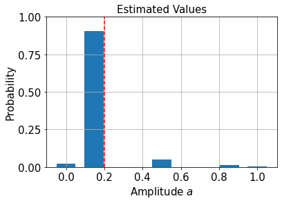
推定値を改善するために測定確率補完して、この確率分布を生成する最尤推定値を計算することができます。
[10]:
print("Interpolated MLE estimator:", ae_result.mle)
Interpolated MLE estimator: 0.19999999406856905
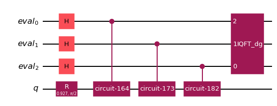
振幅推定が実行する回路を見ることができます。
[11]:
ae_circuit = ae.construct_circuit(problem)
ae_circuit.decompose().draw(
    "mpl", style="iqx"
)  # decompose 1 level: exposes the Phase estimation circuit!
[11]:
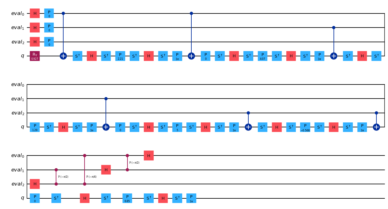
[12]:
from qiskit import transpile


basis_gates = ["h", "ry", "cry", "cx", "ccx", "p", "cp", "x", "s", "sdg", "y", "t", "cz"]
transpile(ae_circuit, basis_gates=basis_gates, optimization_level=2).draw("mpl", style="iqx")
[12]:
反復振幅推定#
[2] を参照してください。
[13]:
from qiskit_algorithms import IterativeAmplitudeEstimation

iae = IterativeAmplitudeEstimation(
    epsilon_target=0.01,  # target accuracy
    alpha=0.05,  # width of the confidence interval
    sampler=sampler,
)
iae_result = iae.estimate(problem)

print("Estimate:", iae_result.estimation)
Estimate: 0.2
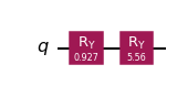
ここでの回路はグローバーの累乗だけで構成されており、はるかに回路コストが低いです。
[14]:
iae_circuit = iae.construct_circuit(problem, k=3)
iae_circuit.draw("mpl", style="iqx")
[14]:
最尤振幅推定#
[3] を参照してください。
[15]:
from qiskit_algorithms import MaximumLikelihoodAmplitudeEstimation

mlae = MaximumLikelihoodAmplitudeEstimation(
    evaluation_schedule=3,  # log2 of the maximal Grover power
    sampler=sampler,
)
mlae_result = mlae.estimate(problem)

print("Estimate:", mlae_result.estimation)
Estimate: 0.20002237175368104
高速振幅推定#
[4] を参照してください。
[18]:
from qiskit_algorithms import FasterAmplitudeEstimation

fae = FasterAmplitudeEstimation(
    delta=0.01,  # target accuracy
    maxiter=3,  # determines the maximal power of the Grover operator
    sampler=sampler,
)
fae_result = fae.estimate(problem)

print("Estimate:", fae_result.estimation)
Estimate: 0.2030235918323876
参考文献#
[1] Quantum Amplitude Amplification and Estimation. Brassard et al (2000). https://arxiv.org/abs/quant-ph/0005055
[2] Iterative Quantum Amplitude Estimation. Grinko, D., Gacon, J., Zoufal, C., & Woerner, S. (2019). https://arxiv.org/abs/1912.05559
[3] Amplitude Estimation without Phase Estimation. Suzuki, Y., Uno, S., Raymond, R., Tanaka, T., Onodera, T., & Yamamoto, N. (2019). https://arxiv.org/abs/1904.10246
[4] Faster Amplitude Estimation. K. Nakaji (2020). https://arxiv.org/pdf/2003.02417.pdf
[17]:
import qiskit.tools.jupyter

%qiskit_version_table
%qiskit_copyright
Version Information
| Software | Version |
|---|---|
qiskit | None |
qiskit-terra | 0.45.0.dev0+c626be7 |
qiskit_ibm_provider | 0.6.1 |
qiskit_algorithms | 0.2.0 |
| System information | |
| Python version | 3.9.7 |
| Python compiler | GCC 7.5.0 |
| Python build | default, Sep 16 2021 13:09:58 |
| OS | Linux |
| CPUs | 2 |
| Memory (Gb) | 5.778430938720703 |
| Fri Aug 18 15:44:17 2023 EDT | |
This code is a part of Qiskit
© Copyright IBM 2017, 2023.
This code is licensed under the Apache License, Version 2.0. You may
obtain a copy of this license in the LICENSE.txt file in the root directory
of this source tree or at http://www.apache.org/licenses/LICENSE-2.0.
Any modifications or derivative works of this code must retain this
copyright notice, and modified files need to carry a notice indicating
that they have been altered from the originals.
[ ]: