Restless Measurements

When running circuits, the qubits are typically reset to the ground state after each measurement to ensure that the next circuit has a well-defined initial state. This can be done passively by waiting several \(T_1\)-times so that qubits in the excited state decay to \(\left\vert0\right\rangle\). Since \(T_1\)-times are continuously improving (they already increased beyond \(100\,\mu s\)), this initialization procedure is now inefficient. This makes active reset necessary. Active qubit reset, as employed by IBM Quantum systems is more efficient and saves time but also lasts a few microseconds (between \(3\) and \(5\,\mu s\)). Furthermore, a delay, typically lasting \(250\,\mu s\), after the reset operation is often necessary to ensure a high initialization quality. However, for several types of characterization and calibration experiments we can avoid qubit reset by post-processing the measurement outcomes and continue directly with the next circuit after an optional short delay, even if the qubit was measured in the excited state. Foregoing qubit reset is the main idea behind restless measurements.

The IBM Quantum systems have dynamical repetition delays enabled. We can thus choose the delay between the execution of two quantum circuits. This delay typically ranges from \(0\) to \(500\,\mu s\) depending on the system. The default value for most devices is \(250\,\mu s\). Restless measurements set this delay to small values such as \(1\,\mu s\) or lower. Note that sometimes the measurement instructions already contain a delay after the measurement pulse to allow the readout resonator to depopulate.

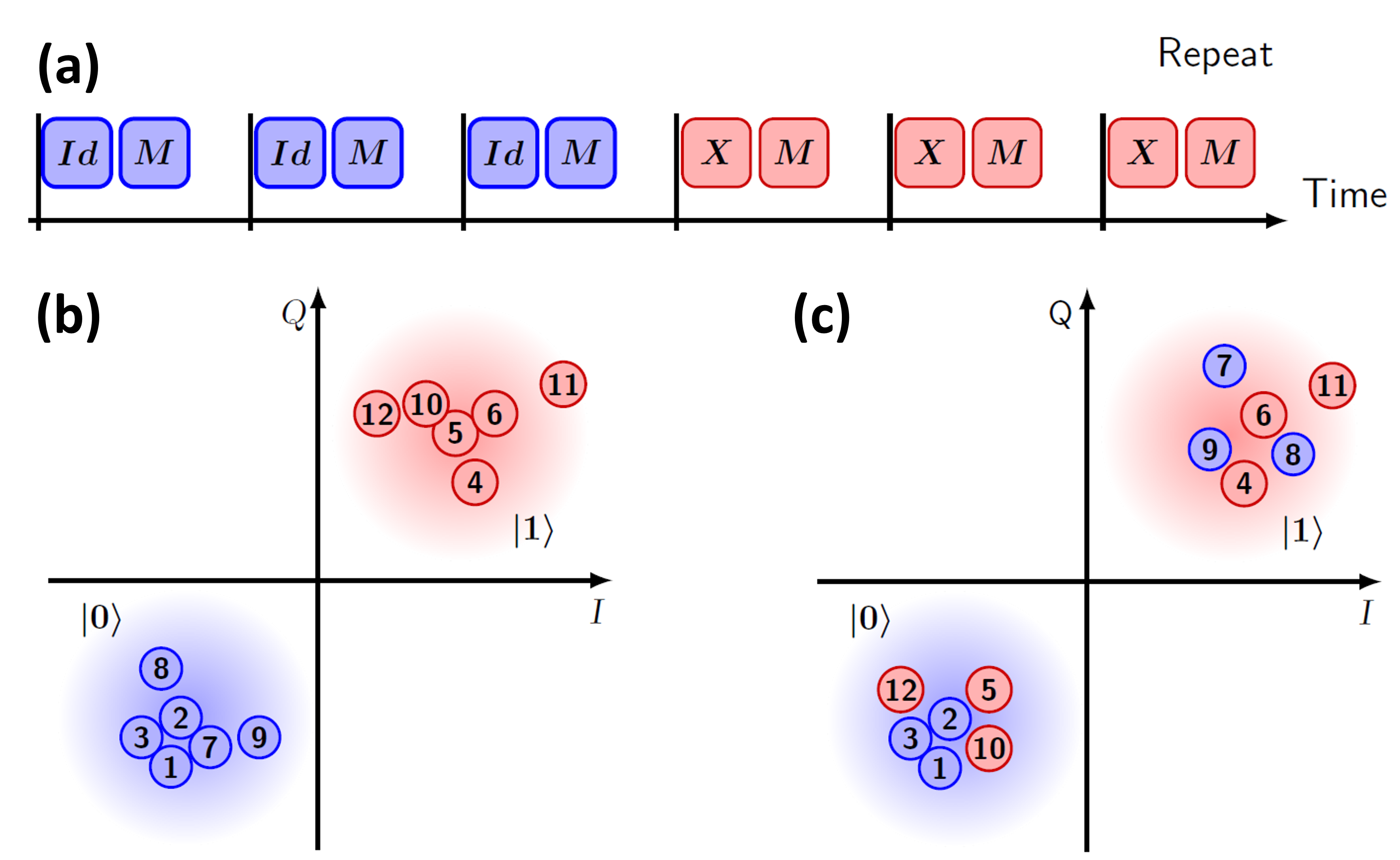
When the qubit is not reset it will either be in the \(\left\vert0\right\rangle\) or in the \(\left\vert1\right\rangle\) state when the next circuit starts. Therefore, the measured outcomes of the restless experiments require post-processing. The following example, taken from Ref. [1], illustrates what happens to the single measurement outcomes represented as complex numbers in the IQ plane in a restless setting. Here, we run three circuits with an identity gate and three circuits with an \(X\) gate, each followed by a measurement. The numbers in the IQ shots indicate the order in which the shots were acquired. The IQ plane on the left shows the single measurement shots gathered when the qubits are reset. Here, the blue and red points, corresponding to measurements following the \(Id\) and \(X\) gates, are associated with the \(\left\vert0\right\rangle\) and \(\left\vert1\right\rangle\) states, respectively. By contrast, with restless measurements the qubit is not reset after a measurement. As one can see in the IQ plane on the right the single measurement outcomes of the \(Id`\) and \(X\) circuits no longer match with the \(\left\vert0\right\rangle\) and \(\left\vert1\right\rangle\) states, respectively. This is why restless measurements need special post-processing.

Enabling restless measurements

In Qiskit Experiments, the experiments that support restless measurements have a special method enable_restless() to set the restless run options and define the data processor that will process the measured data. If you are an experiment developer, you can add the RestlessMixin to your experiment class to add support for restless measurements. Here, we will show how to activate restless measurements using a fake backend and a rough DRAG experiment. Note however, that you will not observe any meaningful outcomes with fake backends since the circuit simulator they use always starts with the qubits in the ground state.

Note

This tutorial requires the qiskit-ibm-runtime package to model a backend. You can install it with python -m pip install qiskit-ibm-runtime.

from qiskit_ibm_runtime.fake_provider import FakePerth

from qiskit_experiments.library import RoughDragCal
from qiskit_experiments.calibration_management import (
    Calibrations,
    FixedFrequencyTransmon,
)
from qiskit_experiments.data_processing.data_processor import DataProcessor

# replace this lines with an IBM Quantum backend to run the experiment.
backend = FakePerth()
cals = Calibrations.from_backend(backend, libraries=[FixedFrequencyTransmon()])

# Define the experiment
qubit = 2
cal_drag = RoughDragCal((qubit,), cals, schedule_name='sx', backend=backend)

# Enable restless measurements by setting the run options and data processor
cal_drag.enable_restless(rep_delay=1e-6)

print(cal_drag.analysis.options.data_processor)
print(cal_drag.run_options)

DataProcessor(input_key=memory, nodes=[RestlessToCounts(validate=True), Probability(validate=True, outcome=1, alpha_prior=[0.5, 0.5])])
Options(meas_level=<MeasLevel.CLASSIFIED: 2>, rep_delay=1e-06, init_qubits=False, memory=True, meas_return=<MeasReturnType.SINGLE: 'single'>, use_measure_esp=False)

As you can see, a restless data processor is automatically chosen for the experiment. This data processor post-processes the restless measured shots according to the order in which they were acquired. Furthermore, the appropriate run options are also set. Note that these run options might be unique to IBM Quantum providers. Therefore, execute may fail on non-IBM Quantum providers if the required options are not supported.

After calling enable_restless() the experiment is ready to be run in a restless mode. With a hardware backend, this would be done by calling the run() method:

drag_data_restless = cal_drag.run()

As shown by the example, the code is identical to running a normal experiment aside from a call to the method enable_restless(). Note that you can also choose to keep the standard data processor by providing it to the analysis options and telling enable_restless() not to override the data processor.

from qiskit_experiments.data_processing import (
    DataProcessor,
    Probability,
)

# define a standard data processor.
standard_processor = DataProcessor("counts", [Probability("1")])

cal_drag = RoughDragCal((qubit,), cals, schedule_name='sx', backend=backend)
cal_drag.analysis.set_options(data_processor=standard_processor)

# enable restless mode and set override_processor_by_restless to False.
cal_drag.enable_restless(rep_delay=1e-6, override_processor_by_restless=False)

If you run the experiment in this setting you will see that the data is often unusable which illustrates the importance of the data processing. As detailed in Ref. [2], restless measurements can be done with a wide variety of experiments such as fine amplitude and drag error amplifying gate sequences as well as randomized benchmarking.

Calculating restless quantum processor speed-ups

Following Ref. [2], we can compare the time spent by the quantum processor executing restless and standard jobs. This allows us to compute the effective speed-up we gain when performing restless experiments. Note that we do not consider any classical run-time contributions such as runtime-compilation or data transfer times [3]. The time to run \(K\) circuits and gather \(N\) shots for each circuit is

\[\tau^{(x)} = NK\left(\tau^{(x)}_\text{reset}+\tau^{(x)}_\text{delay}+ \langle{\tau}_\text{circ}\rangle+\tau_\text{meas}\right),\]

where \(\tau^{(x)}_\text{reset}\) and \(\tau^{(x)}_\text{delay}\) are the reset and post measurement delay times, respectively. The superscript \((x)\) indicates restless \((r)\) or standard \((s)\) measurements. The average duration of all \(K\) circuits in an experiment is \(\langle{\tau}_\text{circ}\rangle=K^{-1}\sum_{k=1}^{K} \tau_{\text{circ},k}\) where \(\tau_{\text{circ},k}\) is the duration of only the gates in circuit \(k\). We therefore compute the quantum processor speed-up of restless measurements as \(\tau^{(\text{s})}/\tau^{(\text{r})}\) which is independent of the number of circuits and shots.

We approximate the standard reset time in IBM Quantum backends by \(\tau^{(s)}_\text{reset} = 4\,\mu s\) whereas \(\tau^{(r)}_\text{reset} = 0\,\mu s\) since we do not reset the qubit in a restless experiment. By default, the repetition delay is \(\tau^{(s)}_\text{delay} = 250\,\mu s\). For our restless experiments we set \(\tau^{(r)}_\text{delay} = 1\,\mu s\). These speed-ups can be evaluated using the code below.

from qiskit import schedule, transpile
from qiskit_experiments.framework import BackendData

dt = BackendData(backend).dt
inst_map = backend.instruction_schedule_map
meas_length = inst_map.get("measure", (qubit,)).duration * dt

# Compute the average duration of all circuits
# Remove measurement instructions
circuits = []
for qc in cal_drag.circuits():
    qc.remove_final_measurements(inplace=True)
    circuits.append(qc)

# Schedule the circuits to obtain the duration of all the gates
executed_circs = transpile(
    circuits,
    backend,
    initial_layout=[qubit],
    scheduling_method="alap",
    **cal_drag.transpile_options.__dict__,
)
durations = [c.duration for c in executed_circs]

tau = sum(durations) * dt / (len(durations))

n_circs = len(cal_drag.circuits())
# can be obtained from backend.default_rep_delay on a backend from qiskit-ibm-provider

delay_s = 0.0025
delay_r = 1e-6  # restless delay
reset = 4e-6  # Estimated reset duration
speed_up = (meas_length + reset + delay_s + tau) / (meas_length + delay_r + tau)
print(f"The QPU will spend {speed_up:.1f}x less time running restless Drag.")

The QPU will spend 1326.1x less time running restless Drag.

The example above is applicable to other experiments and shows that restless measurements can greatly speed-up characterization and calibration tasks.

References

[1]

Max Werninghaus, Daniel J. Egger, Stefan Filipp, High-speed calibration and characterization of superconducting quantum processors without qubit reset, PRX Quantum 2, 020324 (2021). https://arxiv.org/abs/2010.06576.

[2] (1,2)

Caroline Tornow, Naoki Kanazawa, William E. Shanks, Daniel J. Egger, Minimum quantum run-time characterization and calibration via restless measurements with dynamic repetition rates, Physics Review Applied 17, 064061 (2022). https://arxiv.org/abs/2202.06981.

[3]

Andrew Wack, Hanhee Paik, Ali Javadi-Abhari, Petar Jurcevic, Ismael Faro, Jay M. Gambetta, Blake R. Johnson, Quality, Speed, and Scale: three key attributes to measure the performance of near-term quantum computers, https://arxiv.org/abs/2110.14108.

See also

• API documentation: RestlessMixin