Readout Mitigation#
Readout errors affect quantum computation during the measurement of the qubits in a quantum device. By characterizing the readout errors, it is possible to construct a readout error mitigator that is used both to obtain a more accurate distribution of the outputs, and more accurate measurements of expectation value for measurables.
The readout mitigator is generated from an assignment matrix: a \(2^n \times 2^n\) matrix \(A\) such that \(A_{y,x}\) is the probability to observe \(y\) given the true outcome should be \(x\). The assignment matrix is used to compute the mitigation matrix used in the readout error mitigation process itself.
A Local readout mitigator works under the assumption that readout
errors are mostly local, meaning readout errors for different qubits
are independent of each other. In this case, the assignment matrix is
the tensor product of \(n\) \(2 \times 2\) matrices, one for
each qubit, making it practical to store the assignment matrix in
implicit form, by storing the individual \(2 \times 2\) assignment
matrices. The corresponding class in Qiskit is the
LocalReadoutMitigator.
A Correlated readout mitigator uses the full \(2^n \times 2^n\)
assignment matrix, meaning it can only be used for small values of
\(n\). The corresponding class in Qiskit is the
CorrelatedReadoutMitigator.
This notebook demonstrates the usage of both the local and correlated experiments to generate the corresponding mitigators.
Note
This tutorial requires the qiskit-aer and qiskit-ibm-runtime
packages to run simulations. You can install them with python -m pip
install qiskit-aer qiskit-ibm-runtime.
import numpy as np
import matplotlib.pyplot as plt
from qiskit import QuantumCircuit
from qiskit.visualization import plot_distribution
from qiskit_experiments.library import LocalReadoutError, CorrelatedReadoutError

from qiskit_aer import AerSimulator
from qiskit_ibm_runtime.fake_provider import FakePerth

from qiskit.result.mitigation.utils import (
    expval_with_stddev,
    str2diag,
    counts_probability_vector
)

backend = AerSimulator.from_backend(FakePerth())
shots = 1024
qubits = [0,1,2,3]
num_qubits = len(qubits)
Standard mitigation experiment#
The default mitigation experiment is local, meaning error probability is measured individually for each qubit. The experiment generates two circuits, one for all “0” and one for all “1” results.
exp = LocalReadoutError(qubits)
for c in exp.circuits():
    print(c)
         ░ ┌─┐
   q_0: ─░─┤M├─────────
         ░ └╥┘┌─┐
   q_1: ─░──╫─┤M├──────
         ░  ║ └╥┘┌─┐
   q_2: ─░──╫──╫─┤M├───
         ░  ║  ║ └╥┘┌─┐
   q_3: ─░──╫──╫──╫─┤M├
         ░  ║  ║  ║ └╥┘
meas: 4/════╩══╩══╩══╩═
            0  1  2  3
        ┌───┐ ░ ┌─┐
   q_0: ┤ X ├─░─┤M├─────────
        ├───┤ ░ └╥┘┌─┐
   q_1: ┤ X ├─░──╫─┤M├──────
        ├───┤ ░  ║ └╥┘┌─┐
   q_2: ┤ X ├─░──╫──╫─┤M├───
        ├───┤ ░  ║  ║ └╥┘┌─┐
   q_3: ┤ X ├─░──╫──╫──╫─┤M├
        └───┘ ░  ║  ║  ║ └╥┘
meas: 4/═════════╩══╩══╩══╩═
                 0  1  2  3
exp.analysis.set_options(plot=True)
result = exp.run(backend)
mitigator = result.analysis_results("Local Readout Mitigator").value
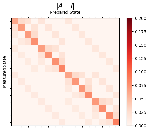
The resulting measurement matrix can be illustrated by comparing it to the identity.
result.figure(0)
Mitigation matrices#
The individual mitigation matrices can be read off the mitigator.
for m in mitigator._mitigation_mats:
    print(m)
    print()
[[ 1.02263374 -0.0308642 ]
 [-0.02263374  1.0308642 ]]

[[ 1.0141844  -0.02330294]
 [-0.0141844   1.02330294]]

[[ 1.01311806 -0.02018163]
 [-0.01311806  1.02018163]]

[[ 1.01513623 -0.01816347]
 [-0.01513623  1.01816347]]
Mitigation example#
qc = QuantumCircuit(num_qubits)
qc.h(0)
for i in range(1, num_qubits):
    qc.cx(i - 1, i)
qc.measure_all()
counts = backend.run(qc, shots=shots, seed_simulator=42, method="density_matrix").result().get_counts()
unmitigated_probs = {label: count / shots for label, count in counts.items()}
mitigated_quasi_probs = mitigator.quasi_probabilities(counts)
mitigated_stddev = mitigated_quasi_probs._stddev_upper_bound
mitigated_probs = (mitigated_quasi_probs.nearest_probability_distribution().binary_probabilities())
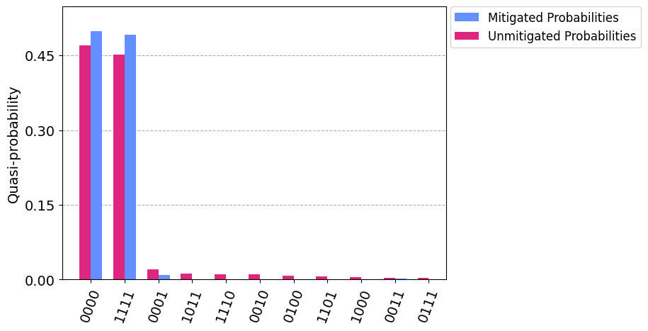
Probabilities#
legend = ['Mitigated Probabilities', 'Unmitigated Probabilities']
plot_distribution([mitigated_probs, unmitigated_probs], legend=legend, sort="value_desc", bar_labels=False)
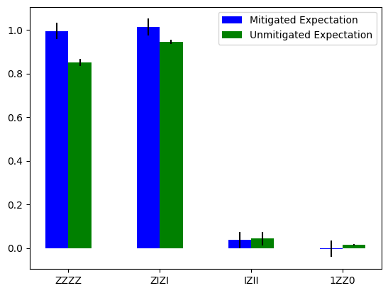
Expectation value#
diagonal_labels = ["ZZZZ", "ZIZI", "IZII", "1ZZ0"]
ideal_expectation = []
diagonals = [str2diag(d) for d in diagonal_labels]
qubit_index = {i: i for i in range(num_qubits)}
unmitigated_probs_vector, _ = counts_probability_vector(unmitigated_probs, qubit_index=qubit_index)
unmitigated_expectation = [expval_with_stddev(d, unmitigated_probs_vector, shots) for d in diagonals]
mitigated_expectation = [mitigator.expectation_value(counts, d) for d in diagonals]
mitigated_expectation_values, mitigated_stddev = zip(*mitigated_expectation)
unmitigated_expectation_values, unmitigated_stddev = zip(*unmitigated_expectation)
legend = ['Mitigated Expectation', 'Unmitigated Expectation']
fig, ax = plt.subplots()
X = np.arange(4)
ax.bar(X + 0.00, mitigated_expectation_values, yerr=mitigated_stddev, color='b', width = 0.25, label="Mitigated Expectation")
ax.bar(X + 0.25, unmitigated_expectation_values, yerr=unmitigated_stddev, color='g', width = 0.25, label="Unmitigated Expectation")
ax.set_xticks([0.125 + i for i in range(len(diagonals))])
ax.set_xticklabels(diagonal_labels)
ax.legend()
<matplotlib.legend.Legend at 0x7fdbb42854c0>
See also#
API documentation:
LocalReadoutError,CorrelatedReadoutErrorQiskit Textbook: Measurement Error Mitigation