Calibrations: Schedules and gate parameters from experiments#
To produce high fidelity quantum operations, we want to be able to run good gates. The calibration module in Qiskit Experiments allows users to run experiments to find the pulse shapes and parameter values that maximize the fidelity of the resulting quantum operations. Calibration experiments encapsulate the internal processes and allow experimenters to perform calibration operations in a quicker way. Without the experiments module, we would need to define pulse schedules and plot the resulting measurement data manually.
In this tutorial, we demonstrate how to calibrate single-qubit gates using the
calibration framework in Qiskit Experiments. We will run experiments on our test pulse
backend, SingleTransmonTestBackend, a backend that simulates the underlying
pulses with qiskit_dynamics on a three-level model of a transmon. You can also
run these experiments on any real backend with Pulse enabled (see
qiskit.providers.models.BackendConfiguration).
We will run experiments to find the qubit frequency, calibrate the amplitude of DRAG pulses, and choose the value of the DRAG parameter that minimizes leakage. The calibration framework requires the user to:
Set up an instance of
Calibrations,Run calibration experiments found in
qiskit_experiments.library.calibration.
Note that the values of the parameters stored in the instance of the Calibrations class
will automatically be updated by the calibration experiments.
This automatic updating can also be disabled using the auto_update flag.
Note
This tutorial requires the qiskit_dynamics package to run simulations.
You can install it with python -m pip install qiskit-dynamics.
import pandas as pd
import numpy as np
import qiskit.pulse as pulse
from qiskit.circuit import Parameter
from qiskit_experiments.calibration_management.calibrations import Calibrations
from qiskit import schedule
from qiskit_experiments.test.pulse_backend import SingleTransmonTestBackend
backend = SingleTransmonTestBackend(5.2e9,-.25e9, 1e9, 0.8e9, noise=False, seed=100)
qubit = 0
cals=Calibrations.from_backend(backend)
print(cals.get_inst_map())
<InstructionScheduleMap(1Q instructions:
Multi qubit instructions:
)>
The two functions below show how to set up an instance of Calibrations.
To do this the user defines the template schedules to calibrate.
These template schedules are fully parameterized, even the channel indices
on which the pulses are played. Furthermore, the name of the parameter in the channel
index must follow the convention laid out in the documentation
of the calibration module. Note that the parameters in the channel indices
are automatically mapped to the channel index when Calibrations.get_schedule() is called.
# A function to instantiate calibrations and add a couple of template schedules.
def setup_cals(backend) -> Calibrations:

    cals = Calibrations.from_backend(backend)

    dur = Parameter("dur")
    amp = Parameter("amp")
    sigma = Parameter("σ")
    beta = Parameter("β")
    drive = pulse.DriveChannel(Parameter("ch0"))

    # Define and add template schedules.
    with pulse.build(name="xp") as xp:
        pulse.play(pulse.Drag(dur, amp, sigma, beta), drive)

    with pulse.build(name="xm") as xm:
        pulse.play(pulse.Drag(dur, -amp, sigma, beta), drive)

    with pulse.build(name="x90p") as x90p:
        pulse.play(pulse.Drag(dur, Parameter("amp"), sigma, Parameter("β")), drive)

    cals.add_schedule(xp, num_qubits=1)
    cals.add_schedule(xm, num_qubits=1)
    cals.add_schedule(x90p, num_qubits=1)

    return cals

# Add guesses for the parameter values to the calibrations.
def add_parameter_guesses(cals: Calibrations):

    for sched in ["xp", "x90p"]:
        cals.add_parameter_value(80, "σ", schedule=sched)
        cals.add_parameter_value(0.5, "β", schedule=sched)
        cals.add_parameter_value(320, "dur", schedule=sched)
        cals.add_parameter_value(0.5, "amp", schedule=sched)
When setting up the calibrations we add three pulses: a \(\pi\)-rotation,
with a schedule named xp, a schedule xm identical to xp
but with a nagative amplitude, and a \(\pi/2\)-rotation, with a schedule
named x90p. Here, we have linked the amplitude of the xp and xm pulses.
Therefore, calibrating the parameters of xp will also calibrate
the parameters of xm.
cals = setup_cals(backend)
add_parameter_guesses(cals)
A similar setup is achieved by using a pre-built library of gates.
The library of gates provides a standard set of gates and some initial guesses
for the value of the parameters in the template schedules.
This is shown below using the FixedFrequencyTransmon library which provides the x,
y, sx, and sy pulses. Note that in the example below
we change the default value of the pulse duration to 320 samples
from qiskit_experiments.calibration_management.basis_gate_library import FixedFrequencyTransmon

library = FixedFrequencyTransmon(default_values={"duration": 320})
cals = Calibrations.from_backend(backend, libraries=[library])
print(library.default_values()) # check what parameter values this library has
print(cals.get_inst_map()) # check the new cals's InstructionScheduleMap made from the library
print(cals.get_schedule('x',(0,))) # check one of the schedules built from the new calibration
[DefaultCalValue(value=320, parameter='duration', qubits=(), schedule_name='x'), DefaultCalValue(value=80.0, parameter='σ', qubits=(), schedule_name='x'), DefaultCalValue(value=0.0, parameter='angle', qubits=(), schedule_name='x'), DefaultCalValue(value=0.5, parameter='amp', qubits=(), schedule_name='x'), DefaultCalValue(value=0.0, parameter='β', qubits=(), schedule_name='x'), DefaultCalValue(value=0.0, parameter='β', qubits=(), schedule_name='sx'), DefaultCalValue(value=320, parameter='duration', qubits=(), schedule_name='sx'), DefaultCalValue(value=80.0, parameter='σ', qubits=(), schedule_name='sx'), DefaultCalValue(value=0.25, parameter='amp', qubits=(), schedule_name='sx'), DefaultCalValue(value=0.0, parameter='angle', qubits=(), schedule_name='sx')]
<InstructionScheduleMap(1Q instructions:
  q0: {'y', 'x', 'sx', 'sy'}
Multi qubit instructions:
)>
ScheduleBlock(Play(Drag(duration=320, sigma=80, beta=0, amp=0.5, angle=0), DriveChannel(0)), name="x", transform=AlignLeft())
We are going to run the spectroscopy, Rabi, DRAG, and fine amplitude calibration experiments one after another and update the parameters after every experiment, keeping track of parameter values.
Finding qubits with spectroscopy#
Here, we are using a backend for which we already know the qubit frequency. We will therefore use the spectroscopy experiment to confirm that there is a resonance at the qubit frequency reported by the backend.
from qiskit_experiments.library.calibration.rough_frequency import RoughFrequencyCal
We first show the contents of the calibrations for qubit 0.
Note that the guess values that we added before apply to all qubits on the chip.
We see this in the table below as an empty tuple () in the qubits column.
Observe that the parameter values of y do not appear in this table as they are given by the values of x.
columns_to_show = ["parameter", "qubits", "schedule", "value", "date_time"]
pd.DataFrame(**cals.parameters_table(qubit_list=[qubit, ()]))[columns_to_show]
| parameter | qubits | schedule | value | date_time | |
|---|---|---|---|---|---|
| 0 | σ | () | sx | 8.00000e+01 | 2024-04-10 21:04:42.... |
| 1 | angle | () | sx | 0.00000e+00 | 2024-04-10 21:04:42.... |
| 2 | drive_freq | (0,) | None | 5.20000e+09 | 2024-04-10 21:04:42.... |
| 3 | amp | () | x | 5.00000e-01 | 2024-04-10 21:04:42.... |
| 4 | amp | () | sx | 2.50000e-01 | 2024-04-10 21:04:42.... |
| 5 | meas_freq | (0,) | None | 0.00000e+00 | 2024-04-10 21:04:42.... |
| 6 | β | () | x | 0.00000e+00 | 2024-04-10 21:04:42.... |
| 7 | β | () | sx | 0.00000e+00 | 2024-04-10 21:04:42.... |
| 8 | duration | () | x | 3.20000e+02 | 2024-04-10 21:04:42.... |
| 9 | angle | () | x | 0.00000e+00 | 2024-04-10 21:04:42.... |
| 10 | duration | () | sx | 3.20000e+02 | 2024-04-10 21:04:42.... |
| 11 | σ | () | x | 8.00000e+01 | 2024-04-10 21:04:42.... |
Instantiate the experiment and draw the first circuit in the sweep:
freq01_estimate = backend.defaults().qubit_freq_est[qubit]
frequencies = np.linspace(freq01_estimate-15e6, freq01_estimate+15e6, 51)
spec = RoughFrequencyCal((qubit,), cals, frequencies, backend=backend)
spec.set_experiment_options(amp=0.005)
circuit = spec.circuits()[0]
circuit.draw(output="mpl", style="iqp")
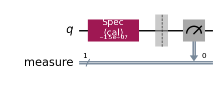
We can also visualize the pulse schedule for the circuit:
next(iter(circuit.calibrations["Spec"].values())).draw()
circuit.calibrations["Spec"]
{((0,),
  (-15000000.0,)): ScheduleBlock(ShiftFrequency(-15000000, DriveChannel(0)), Play(GaussianSquare(duration=2400, sigma=599.9999999999999, width=0.0, amp=0.005, angle=0.0), DriveChannel(0)), ShiftFrequency(15000000, DriveChannel(0)), name="spectroscopy", transform=AlignLeft())}
Run the calibration experiment:
spec_data = spec.run().block_for_results()
spec_data.figure(0)
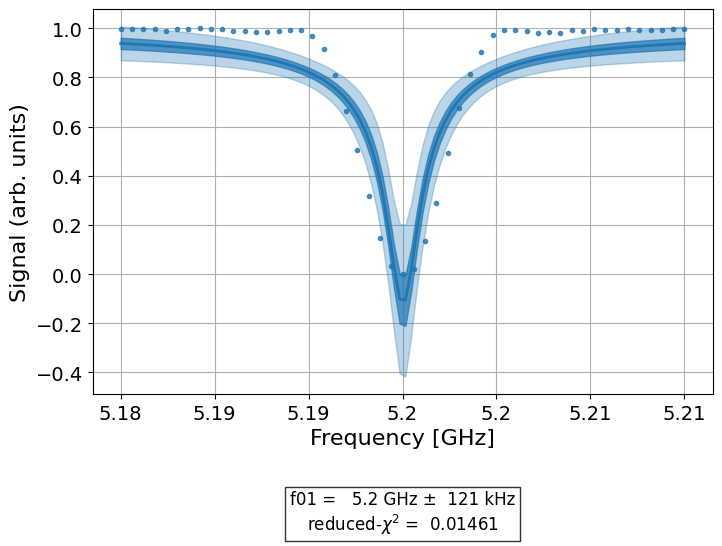
print(spec_data.analysis_results("f01"))
AnalysisResult
- name: f01
- value: (5.20002+/-0.00012)e+09
- χ²: 0.01460755458541581
- quality: good
- extra: <3 items>
- device_components: ['Q0']
- verified: False
The instance of calibrations has been automatically updated with the measured
frequency, as shown below. In addition to the columns shown below, calibrations also
stores the group to which a value belongs, whether a value is valid or not, and the
experiment id that produced a value.
pd.DataFrame(**cals.parameters_table(qubit_list=[qubit]))[columns_to_show]
| parameter | qubits | schedule | value | date_time | |
|---|---|---|---|---|---|
| 0 | meas_freq | (0,) | None | 0.00000e+00 | 2024-04-10 21:04:42.... |
| 1 | drive_freq | (0,) | None | 5.20002e+09 | 2024-04-10 21:05:09.... |
Calibrating the pulse amplitudes with a Rabi experiment#
In the Rabi experiment we apply a pulse at the frequency of the qubit
and scan its amplitude to find the amplitude that creates a rotation
of a desired angle. We do this with the calibration experiment RoughXSXAmplitudeCal.
This is a specialization of the Rabi experiment that will update the calibrations
for both the \(X\) pulse and the \(SX\) pulse using a single experiment.
from qiskit_experiments.library.calibration import RoughXSXAmplitudeCal
rabi = RoughXSXAmplitudeCal((qubit,), cals, backend=backend, amplitudes=np.linspace(-0.1, 0.1, 51))
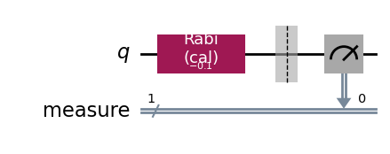
The rough amplitude calibration is therefore a Rabi experiment in which each circuit contains a pulse with a gate. Different circuits correspond to pulses with different amplitudes.
rabi.circuits()[0].draw(output="mpl", style="iqp")
After the experiment completes the value of the amplitudes in the calibrations
will automatically be updated. This behaviour can be controlled using the auto_update
argument given to the calibration experiment at initialization.
rabi_data = rabi.run().block_for_results()
rabi_data.figure(0)
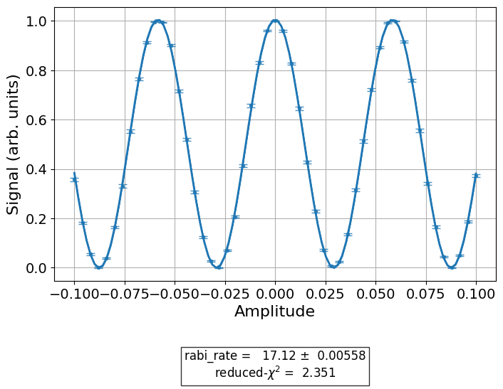
print(rabi_data.analysis_results("rabi_rate"))
AnalysisResult
- name: rabi_rate
- value: 17.115+/-0.006
- χ²: 2.3507719247367604
- quality: bad
- extra: <2 items>
- device_components: ['Q0']
- verified: False
pd.DataFrame(**cals.parameters_table(qubit_list=[qubit, ()], parameters="amp"))[columns_to_show]
| parameter | qubits | schedule | value | date_time | |
|---|---|---|---|---|---|
| 0 | amp | (0,) | x | 0.02921 | 2024-04-10 21:05:24.... |
| 1 | amp | () | sx | 0.25000 | 2024-04-10 21:04:42.... |
| 2 | amp | (0,) | sx | 0.01461 | 2024-04-10 21:05:24.... |
| 3 | amp | () | x | 0.50000 | 2024-04-10 21:04:42.... |
The table above shows that we have now updated the amplitude of our \(\pi\) pulse
from 0.5 to the value obtained in the most recent Rabi experiment.
Importantly, since we linked the amplitudes of the x and y schedules
we will see that the amplitude of the y schedule has also been updated
as seen when requesting schedules from the Calibrations instance.
Furthermore, we used the result from the Rabi experiment to also update
the value of the sx pulse.
cals.get_schedule("sx", qubit)
ScheduleBlock(Play(Drag(duration=320, sigma=80, beta=0, amp=0.01460699, angle=0), DriveChannel(0)), name="sx", transform=AlignLeft())
cals.get_schedule("x", qubit)
ScheduleBlock(Play(Drag(duration=320, sigma=80, beta=0, amp=0.02921398, angle=0), DriveChannel(0)), name="x", transform=AlignLeft())
cals.get_schedule("y", qubit)
ScheduleBlock(Play(Drag(duration=320, sigma=80, beta=0, amp=0.02921398, angle=1.5707963268), DriveChannel(0)), name="y", transform=AlignLeft())
Saving and loading calibrations#
The values of the calibrated parameters can be saved to a .csv file and reloaded at a later point in time.
cals.save(file_type="csv", overwrite=True, file_prefix="PulseBackend")
After saving the values of the parameters you may restart your kernel. If you do so,
you will only need to run the following cell to recover the state of your calibrations.
Since the schedules are currently not stored we need to call our setup_cals function
or use a library to populate an instance of Calibrations with the template schedules.
By contrast, the value of the parameters will be recovered from the file.
cals = Calibrations.from_backend(backend, library)
cals.load_parameter_values(file_name="PulseBackendparameter_values.csv")
pd.DataFrame(**cals.parameters_table(qubit_list=[qubit, ()], parameters="amp"))[columns_to_show]
| parameter | qubits | schedule | value | date_time | |
|---|---|---|---|---|---|
| 0 | amp | (0,) | x | 0.02921 | 2024-04-10 21:05:24.... |
| 1 | amp | () | sx | 0.25000 | 2024-04-10 21:04:42.... |
| 2 | amp | (0,) | sx | 0.01461 | 2024-04-10 21:05:24.... |
| 3 | amp | () | x | 0.50000 | 2024-04-10 21:04:42.... |
Calibrating the value of the DRAG coefficient#
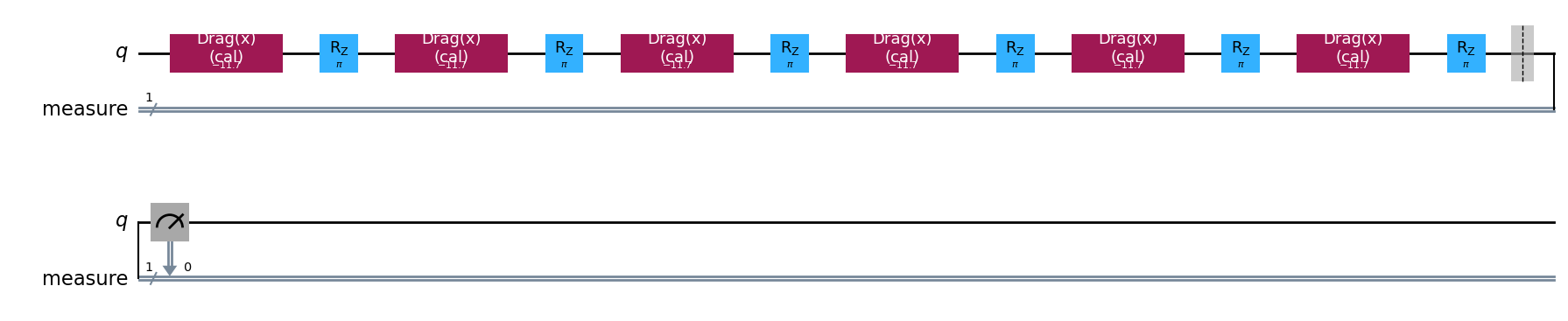
A Derivative Removal by Adiabatic Gate (DRAG) pulse is designed to minimize leakage and phase errors to a neighbouring transition. It is a standard pulse with an additional derivative component. It is designed to reduce the frequency spectrum of a normal pulse near the \(|1\rangle - |2\rangle\) transition, reducing the chance of leakage to the \(|2\rangle\) state. The optimal value of the DRAG parameter is chosen to minimize both leakage and phase errors resulting from the AC Stark shift. The pulse envelope is \(f(t)=\Omega_x(t)+j\beta\frac{\rm d}{{\rm d}t}\Omega_x(t)\). Here, \(\Omega_x(t)\) is the envelop of the in-phase component of the pulse and \(\beta\) is the strength of the quadrature which we refer to as the DRAG parameter and seek to calibrate in this experiment. The DRAG calibration will run several series of circuits. In a given circuit a Rp(β) - Rm(β) block is repeated \(N\) times. Here, Rp is a rotation with a positive angle and Rm is the same rotation with a negative amplitude.
from qiskit_experiments.library import RoughDragCal
cal_drag = RoughDragCal([qubit], cals, backend=backend, betas=np.linspace(-20, 20, 25))
cal_drag.set_experiment_options(reps=[3, 5, 7])
cal_drag.circuits()[5].draw(output="mpl", style="iqp")
drag_data = cal_drag.run().block_for_results()
drag_data.figure(0)
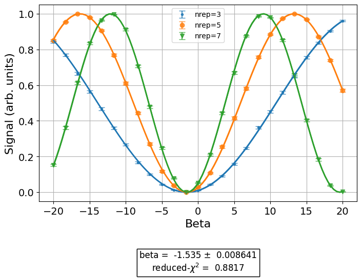
print(drag_data.analysis_results("beta"))
AnalysisResult
- name: beta
- value: -1.535+/-0.009
- χ²: 0.8817188143346306
- quality: bad
- extra: <2 items>
- device_components: ['Q0']
- verified: False
pd.DataFrame(**cals.parameters_table(qubit_list=[qubit, ()], parameters="β"))[columns_to_show]
| parameter | qubits | schedule | value | date_time | |
|---|---|---|---|---|---|
| 0 | β | () | sx | 0.00000 | 2024-04-10 21:04:42.... |
| 1 | β | (0,) | x | -1.53463 | 2024-04-10 21:05:28.... |
| 2 | β | () | x | 0.00000 | 2024-04-10 21:04:42.... |
Fine calibrations of a pulse amplitude#
The amplitude of a pulse can be precisely calibrated using error amplifying gate
sequences. These gate sequences apply the same gate a variable number of times.
Therefore, if each gate has a small error \(d\theta\) in the rotation angle then a
sequence of \(n\) gates will have a rotation error of \(n\) * \(d\theta\).
The FineAmplitude experiment and its subclass experiments implements these
sequences to obtain the correction value of imperfect pulses. We will first examine how
to detect imperfect pulses using the characterization version of these experiments, then
update calibrations with a calibration experiment.
from qiskit.pulse import InstructionScheduleMap
from qiskit_experiments.library import FineXAmplitude
Detecting over- and under-rotated pulses#
We now run the error amplifying experiments with our own pulse schedules on which we
purposefully add over- and under-rotations to observe their effects. To do this, we
create an instruction to schedule map which we populate with the schedules we wish to
work with. This instruction schedule map is then given to the transpile options of the
experiment so that the Qiskit transpiler can attach the pulse schedules to the gates in
the experiments. We base all our pulses on the default \(X\) pulse of
SingleTransmonTestBackend.
x_pulse = backend.defaults().instruction_schedule_map.get('x', (qubit,)).instructions[0][1].pulse
d0, inst_map = pulse.DriveChannel(qubit), pulse.InstructionScheduleMap()
We now take the ideal \(X\) pulse amplitude reported by the backend and add/subtract a 2% over/underrotation to it by scaling the ideal amplitude and see if the experiment can detect this over/underrotation. We replace the default \(X\) pulse in the instruction schedule map with this over/under-rotated pulse.
ideal_amp = x_pulse.amp
over_amp = ideal_amp*1.02
under_amp = ideal_amp*0.98
print(f"The reported amplitude of the X pulse is {ideal_amp:.4f} which we set as ideal_amp.")
print(f"we use {over_amp:.4f} amplitude for overrotation pulse and {under_amp:.4f} for underrotation pulse.")
# build the over rotated pulse and add it to the instruction schedule map
with pulse.build(backend=backend, name="x") as x_over:
    pulse.play(pulse.Drag(x_pulse.duration, over_amp, x_pulse.sigma, x_pulse.beta), d0)
inst_map.add("x", (qubit,), x_over)
The reported amplitude of the X pulse is 0.0582 which we set as ideal_amp.
we use 0.0594 amplitude for overrotation pulse and 0.0570 for underrotation pulse.
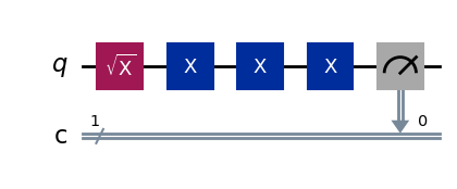
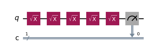
Let’s look at one of the circuits of the FineXAmplitude experiment. To
calibrate the \(X\) gate, we add an \(SX\) gate before the \(X\) gates to
move the ideal population to the equator of the Bloch sphere where the sensitivity to
over/under rotations is the highest.
overamp_exp = FineXAmplitude((qubit,), backend=backend)
overamp_exp.set_transpile_options(inst_map=inst_map)
overamp_exp.circuits()[4].draw(output="mpl", style="iqp")
# do the experiment
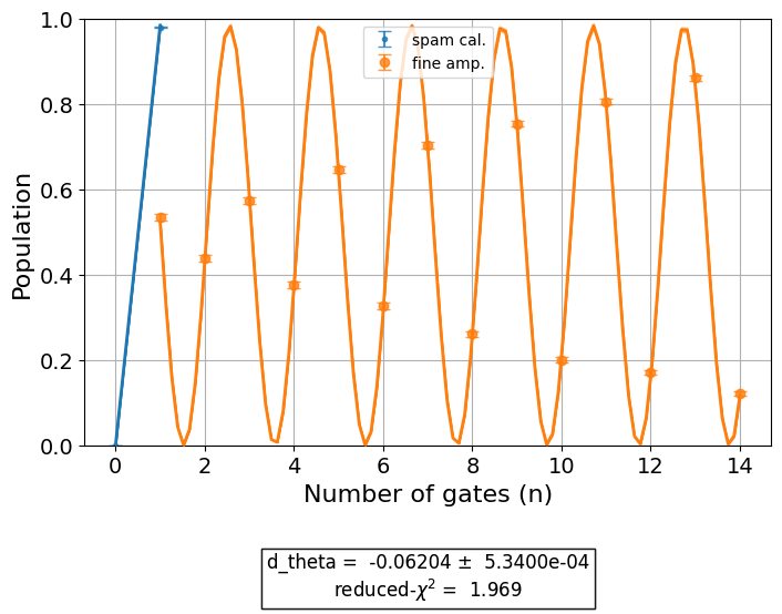
exp_data_over = overamp_exp.run(backend).block_for_results()
exp_data_over.figure(0)
The ping-pong pattern on the figure indicates an over-rotation which makes the initial state rotate more than \(\pi\).
We now look at a pulse with an under rotation to see how the FineXAmplitude
experiment detects this error. We will compare the results to the over-rotation above.
# build the under rotated pulse and add it to the instruction schedule map
with pulse.build(backend=backend, name="x") as x_under:
    pulse.play(pulse.Drag(x_pulse.duration, under_amp, x_pulse.sigma, x_pulse.beta), d0)
inst_map.add("x", (qubit,), x_under)

# do the experiment
underamp_exp = FineXAmplitude((qubit,), backend=backend)
underamp_exp.set_transpile_options(inst_map=inst_map)

exp_data_under = underamp_exp.run(backend).block_for_results()
exp_data_under.figure(0)
Similarly to the over-rotation, the under-rotated pulse creates qubit populations that do not lie on the equator of the Bloch sphere. However, compared to the ping-pong pattern of the over rotated pulse, the under rotated pulse produces an inverted ping-pong pattern. This allows us to determine not only the magnitude of the rotation error but also its sign.
# analyze the results
target_angle = np.pi
dtheta_over = exp_data_over.analysis_results("d_theta").value.nominal_value
scale_over = target_angle / (target_angle + dtheta_over)
dtheta_under = exp_data_under.analysis_results("d_theta").value.nominal_value
scale_under = target_angle / (target_angle + dtheta_under)
print(f"The ideal angle is {target_angle:.2f} rad. We measured a deviation of {dtheta_over:.3f} rad in over-rotated pulse case.")
print(f"Thus, scale the {over_amp:.4f} pulse amplitude by {scale_over:.3f} to obtain {over_amp*scale_over:.5f}.")
print(f"On the other hand, we measured a deviation of {dtheta_under:.3f} rad in under-rotated pulse case.")
print(f"Thus, scale the {under_amp:.4f} pulse amplitude by {scale_under:.3f} to obtain {under_amp*scale_under:.5f}.")
The ideal angle is 3.14 rad. We measured a deviation of 0.065 rad in over-rotated pulse case.
Thus, scale the 0.0594 pulse amplitude by 0.980 to obtain 0.05817.
On the other hand, we measured a deviation of -0.062 rad in under-rotated pulse case.
Thus, scale the 0.0570 pulse amplitude by 1.020 to obtain 0.05820.
Calibrating a \(\pi\)/2 \(X\) pulse#
Now we apply the same principles to a different example using the calibration version of
a Fine Amplitude experiment. The amplitude of the \(SX\) gate, which is an \(X\)
pulse with half the amplitude, is calibrated with the FineSXAmplitudeCal
experiment. Unlike the FineSXAmplitude experiment, the
FineSXAmplitudeCal experiment does not require other gates than the \(SX\)
gate since the number of repetitions can be chosen such that the ideal population is
always on the equator of the Bloch sphere. To demonstrate the
FineSXAmplitudeCal experiment, we create a \(SX\) pulse by dividing the
amplitude of the X pulse by two. We expect that this pulse might have a small rotation
error which we want to correct.
from qiskit_experiments.library import FineSXAmplitudeCal

amp_cal = FineSXAmplitudeCal((qubit,), cals, backend=backend, schedule_name="sx")
amp_cal.circuits()[4].draw(output="mpl", style="iqp")
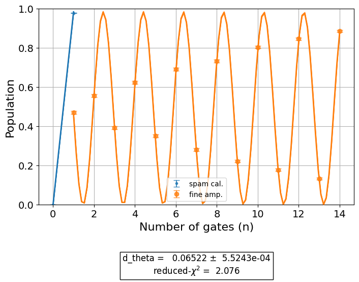
Let’s run the calibration experiment:
exp_data_x90p = amp_cal.run().block_for_results()
exp_data_x90p.figure(0)
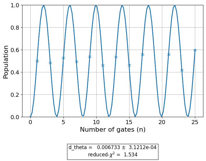
Observe, once again, that the calibrations have automatically been updated.
pd.DataFrame(**cals.parameters_table(qubit_list=[qubit, ()], parameters="amp"))[columns_to_show]
| parameter | qubits | schedule | value | date_time | |
|---|---|---|---|---|---|
| 0 | amp | (0,) | x | 0.02921 | 2024-04-10 21:05:24.... |
| 1 | amp | () | sx | 0.25000 | 2024-04-10 21:04:42.... |
| 2 | amp | (0,) | sx | 0.01454 | 2024-04-10 21:05:31.... |
| 3 | amp | () | x | 0.50000 | 2024-04-10 21:04:42.... |
cals.get_schedule("sx", qubit)
ScheduleBlock(Play(Drag(duration=320, sigma=80, beta=0, amp=0.0145446468, angle=0), DriveChannel(0)), name="sx", transform=AlignLeft())
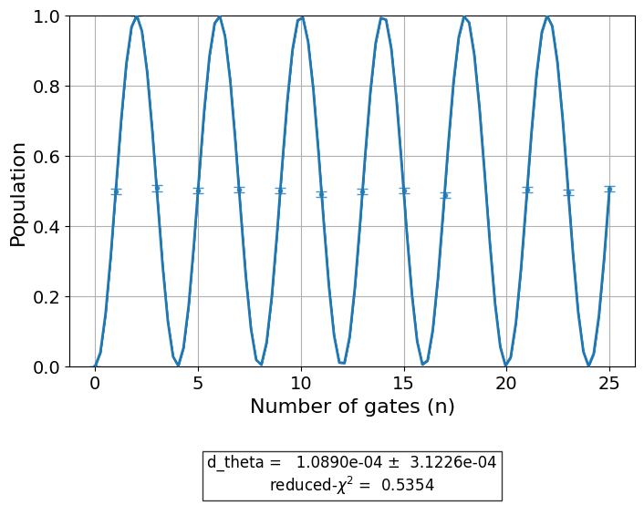
If we run the experiment again, we expect to see that the updated calibrated gate will have a smaller \(d\theta\) error:
exp_data_x90p_rerun = amp_cal.run().block_for_results()
exp_data_x90p_rerun.figure(0)
See also#
API documentation:
calibration_managementandcalibrationQiskit Textbook: Calibrating Qubits with Qiskit Pulse