Curve Analysis: Fitting your data#

For most experiments, we are interested in fitting our results to a pre-defined mathematical model. The Curve Analysis module provides the analysis base class for a variety of experiments with a single experimental parameter sweep. Analysis subclasses can override several class attributes to customize the behavior from data processing to post-processing, including providing systematic initial guesses for parameters tailored to the experiment. Here we describe how the Curve Analysis module works and how you can create new analyses that inherit from the base class.

Curve Analysis overview#

The base class CurveAnalysis implements the multi-objective optimization on different sets of experiment results. A single experiment can define sub-experiments consisting of multiple circuits which are tagged with common metadata, and curve analysis sorts the experiment results based on the circuit metadata.

This is an example showing the abstract data flow of a typical curve analysis experiment:

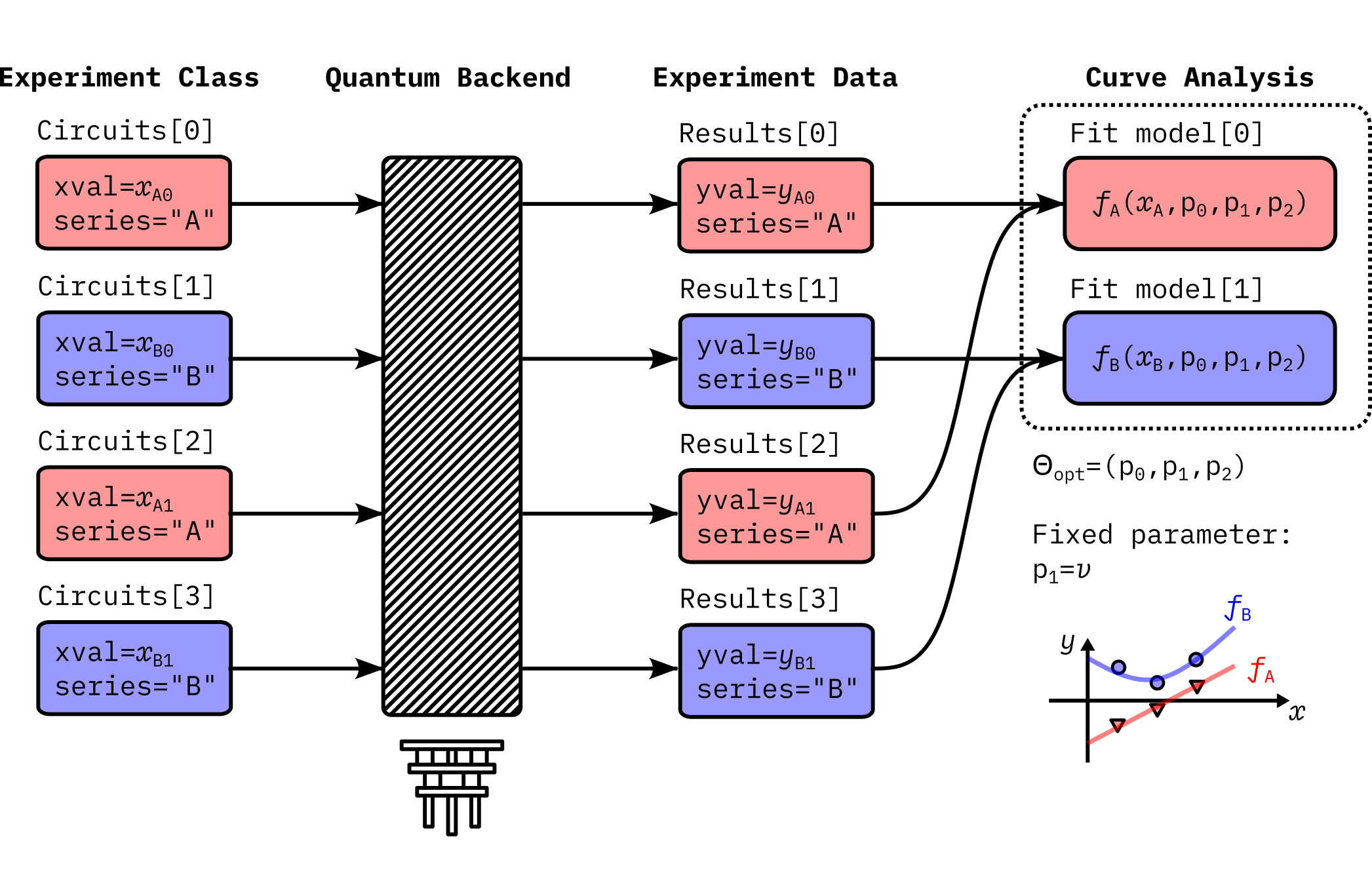
Here the experiment runs two subsets of experiments, namely, series A and series B. The analysis defines corresponding fit models \(f_A(x_A)\) and \(f_B(x_B)\). Data extraction function in the analysis creates two datasets, \((x_A, y_A)\) for the series A and \((x_B, y_B)\) for the series B, from the experiment data. Optionally, the curve analysis can fix certain parameters during the fitting. In this example, \(p_1 = v\) remains unchanged during the fitting.

The curve analysis aims at solving the following optimization problem:

\[\Theta_{\mbox{opt}} = \arg\min_{\Theta_{\rm fit}} \sigma^{-2} (F(X, \Theta)-Y)^2,\]

where \(F\) is the composite objective function defined on the full experiment data \((X, Y)\), where \(X = x_A \oplus x_B\) and \(Y = y_A \oplus y_B\). This objective function can be described by two fit functions as follows.

\[F(X, \Theta) = f_A(x_A, \theta_A) \oplus f_B(x_B, \theta_B).\]

The solver conducts the least square curve fitting against this objective function and returns the estimated parameters \(\Theta_{\mbox{opt}}\) that minimize the reduced chi-squared value. The parameters to be evaluated are \(\Theta = \Theta_{\rm fit} \cup \Theta_{\rm fix}\), where \(\Theta_{\rm fit} = \theta_A \cup \theta_B\). Since series A and B share the parameters in this example, \(\Theta_{\rm fit} = \{p_0, p_2\}\), and the fixed parameters are \(\Theta_{\rm fix} = \{ p_1 \}\) as mentioned. Thus, \(\Theta = \{ p_0, p_1, p_2 \}\).

Experiment for each series can perform individual parameter sweep for \(x_A\) and \(x_B\), and experiment data yields outcomes \(y_A\) and \(y_B\), which might be of different size. Data processing functions may also compute \(\sigma_A\) and \(\sigma_B\), which are the uncertainty of outcomes arising from the sampling error or measurement error.

More specifically, the curve analysis defines the following data model.

Model: Definition of a single curve that is a function of a reserved parameter “x”.
Group: List of models. Fit functions defined under the same group must share the fit parameters. Fit functions in the group are simultaneously fit to generate a single fit result.

Once the group is assigned, a curve analysis instance builds a proper internal optimization routine. Finally, the analysis outputs a set of AnalysisResultData entries for important fit outcomes along with a single figure of the fit curves with the measured data points.

With this base class, a developer can avoid writing boilerplate code in various curve analyses subclasses and can quickly write up the analysis code for a particular experiment.

Defining new models#

The fit model is defined by the LMFIT Model. If you are familiar with this package, you can skip this section. The LMFIT package manages complicated fit functions and offers several algorithms to solve non-linear least-square problems. Curve Analysis delegates the core fitting functionality to this package.

You can intuitively write the definition of a model, as shown below:

import lmfit

models = [
    lmfit.models.ExpressionModel(
        expr="amp * exp(-alpha * x) + base",
        name="exp_decay",
    )
]

Note that x is the reserved name to represent a parameter that is scanned during the experiment. In above example, the fit function consists of three parameters (amp, alpha, base), and exp indicates a universal function in Python’s math module. Alternatively, you can take a callable to define the model object.

import lmfit
import numpy as np

def exp_decay(x, amp, alpha, base):
    return amp * np.exp(-alpha * x) + base

models = [lmfit.Model(func=exp_decay)]

See the LMFIT documentation for detailed user guide. They also provide preset models.

If the CurveAnalysis object is instantiated with multiple models, it internally builds a cost function to simultaneously minimize the residuals of all fit functions. The names of the parameters in the fit function are important since they are used in the analysis result, and potentially in your experiment database as a fit result.

Here is another example on how to implement a multi-objective optimization task:

import lmfit

models = [
    lmfit.models.ExpressionModel(
        expr="amp * exp(-alpha1 * x) + base",
        name="my_experiment1",
    ),
    lmfit.models.ExpressionModel(
        expr="amp * exp(-alpha2 * x) + base",
        name="my_experiment2",
    ),
]

In addition, you need to provide data_subfit_map analysis option, which may look like

data_subfit_map = {
    "my_experiment1": {"tag": 1},
    "my_experiment2": {"tag": 2},
}

This option specifies the metadata of your experiment circuit that is tied to the fit model. If multiple models are provided without this option, the curve fitter cannot prepare the data for fitting. In this model, you have four parameters (amp, alpha1, alpha2, base) and the two curves share amp (base) for the amplitude (baseline) in the exponential decay function. Here one should expect the experiment data will have two classes of data with metadata "tag": 1 and "tag": 2 for my_experiment1 and my_experiment2, respectively.

By using this model, you can flexibly set up your fit model. Here is another example:

import lmfit

models = [
    lmfit.models.ExpressionModel(
        expr="amp * cos(2 * pi * freq * x + phi) + base",
        name="my_experiment1",
    ),
    lmfit.models.ExpressionModel(
        expr="amp * sin(2 * pi * freq * x + phi) + base",
        name="my_experiment2",
    ),
]

You have the same set of fit parameters in the two models, but now you fit two datasets with different trigonometric functions.

Fitting with fixed parameters#

You can also keep certain parameters unchanged during the fitting by specifying the parameter names in the analysis option fixed_parameters. This feature is useful especially when you want to define a subclass of a particular analysis class.

class AnalysisA(CurveAnalysis):

    def __init__(self):
        super().__init__(
            models=[
                lmfit.models.ExpressionModel(
                    expr="amp * exp(-alpha * x) + base", name="my_model"
                )
            ]
        )

class AnalysisB(AnalysisA):

    @classmethod
    def _default_options(cls) -> Options:
        options = super()._default_options()
        options.fixed_parameters = {"amp": 3.0}

        return options

The parameter specified in fixed_parameters is excluded from the fitting. This code will give you identical fit model to the one defined in the following class:

class AnalysisB(CurveAnalysis):

    super().__init__(
        models=[
            lmfit.models.ExpressionModel(
                expr="3.0 * exp(-alpha * x) + base", name="my_model"
            )
        ]
    )

However, note that you can also inherit other features, e.g. the algorithm to generate initial guesses for parameters, from the AnalysisA class in the first example. On the other hand, in the latter case, you need to manually copy and paste every logic defined in AnalysisA.

Managing intermediate data#

ScatterTable is the single source of truth for the data used in curve fit analysis. Curve analysis primarily involves working with curves, which consist of a series of x and y values along with a series of standard error values for the y values. ScatterTable gathers all of the data from all of the curves together into a single table with one row for each x, y value.

Since analysis can involve several curves, a system is needed for labeling them. ScatterTable uses three labels for identifying curves. In order of narrowest to broadest scope, these labels are series (represented by series_id and series_name columns in the table; see below), category, and analysis.

A series is a set of x and y values for which the y values are expected to follow a single function of x with fixed values for any other parameters of the function. For example, a series could consist of x and correpsonding y values for the model a * cos(w * x) for specific a and w values. However, if the data set had values for a = 1 and a = 0.5, it would contain two series rather than one. In the ScatterTable, a series is specified with the series_id (integer) and series_name (string) columns (see below). Some methods like ScatterTable.filter() accept series as an argument that could be either series_name or series_id so we use series when the distinction is not important.
A category is a label for a group of series that correspond to a particular stage of processing. For example, the series data received from quantum circuit execution and prepared for fitting could be labeled with the category “formatted” while the series data produced using fitted model parameters could be labeled with the category “fitted”.
The analysis label holds the name of the CurveAnalysis subclass associated with each series. For a simple CurveAnalysis subclass, all series would have the same analysis label. However, for CompositeCurveAnalysis, multiple CurveAnalysis subclasses can be associated with a single experiment, and this label can help distinguish curves that have the same series and category.

Here we review the default behavior of CurveAnalysis and CompositeCurveAnalysis regarding the assignment of series_id, series_name, category, and analysis.

The data set provided to the analysis by ExperimentData.data() is processed using the DataProcessor set with the data_processor analysis option. When no data_processor option is set, the default behavior is to convert counts to probability for level 2 data. For level 1 data, the default behavior is to project the complex values to real values using singular value decomposition, average the values if individual shot data were returned, and then normalize the results. This processed data set is then given the category “raw”. This data set is classified into series using the data_subfit_map analysis option as described above with the series_name set to the matched key in data_subfit_map (which matches a fit model name) and the series_id set to the corresponding index for that fit model in the CurveAnalysis.models list. If the CurveAnalysis subclass has a single unnamed model, the series_name is set to model-0. If a data point does not match any key, it is given a null value for series_name and series_id. These operations are performed in the CurveAnalysis._run_data_processing() method.

The “raw” data are then fed into the CurveAnalysis._format_data method for which the default behavior is to average all of the y values within a series with the same x value. The formatted data are added to the ScatterTable with the same series labels and the category of “formatted”. The “formatted” data set is then queried from the ScatterTable and passed to the CurveAnalysis._run_curve_fit() method which performs the fitting. Afterward new curves for each series are generated using the fit models and fitting parameters and added to the ScatterTable with the category “fitted”.

The preceding steps are performed by CurveAnalysis and all of the entries in the ScatterTable are given the name of the analysis class for the analysis column. For CompositeCurveAnalysis, the same procedure is repeated for each component CurveAnalysis class and the series are given the name of that class for the analysis column, so the results from different component analysis classes can be distinguished.

Note that ScatterTable.add_row() allows for curve analysis subclasses to set arbitrary values for series_name, series_id, and category as appropriate. An analysis class may override some of the default curve analysis methods and add additional category labels or define other series not named after a model. For example, StarkRamseyXYAmpScanAnalysis defines four series labels in its data_subfit_map option (Xpos, Ypos, Xneg, Yneg) but only two models (FREQpos, FREQneg) whose names do not match the series labels. It does this by overriding the CurveData._format_data() method and adding its own series to the ScatterTable with series labels to match its fit model names (by combining Xpos and Ypos series data into a FREQpos series and similary for the series with names ending with neg). It sets a custom category, “freq”, for its series but also sets the fit_category analysis option to “freq” so that normal curve fitting is performed on this custom "freq" series data.

The (series, category, analysis) triplet can be used to extract data points that belong to a particular categorized series. For example,

mini_table = table.filter(series="my_experiment1", category="raw", analysis="AnalysisA")
mini_x = mini_table.x
mini_y = mini_table.y

This operation is equivalent to

mini_x = table.xvals(series="my_experiment1", category="raw", analysis="AnalysisA")
mini_y = table.yvals(series="my_experiment1", category="raw", analysis="AnalysisA")

When a CurveAnalysis subclass only has a single model and the table is created from a single analysis instance, the series_id and analysis are trivial, and you only need to specify the category to get subset data of interest.

The full description of ScatterTable columns is as follows:

xval: Parameter scanned in the experiment. This value must be defined in the circuit metadata.
yval: Nominal part of the outcome. The outcome is, for example, an expectation value computed from the experiment results with a data processor.
yerr: Standard error of the outcome, which is mainly due to sampling error.
series_name: Human readable name of the data series. This is defined by the data_subfit_map option in the CurveAnalysis.
series_id: Integer corresponding to the name of data series. This number is automatically assigned.
category: A category that could group several series. This is defined by a developer of the CurveAnalysis subclass and usually corresponds to a stage of data processing like “raw” or “formatted”.
shots: Number of measurement shots used to acquire a data point. This value can be defined in the circuit metadata.
analysis: The name of the curve analysis instance that generated a data point.

ScatterTable helps an analysis developer to write a custom analysis class without the overhead of complex data management. It also helps end-users to retrieve and reuse the intermediate data from an experiment in their custom fitting workflow outside our curve fitting framework. Note that a ScatterTable instance may be saved in the ExperimentData as an artifact. See the Artifacts how-to for more information.

Curve Analysis workflow#

Warning

CurveData dataclass is replaced with ScatterTable dataframe. This class will be deprecated and removed in the future release.

Typically curve analysis performs fitting as follows. This workflow is defined in the method CurveAnalysis._run_analysis().

1. Initialization#

Curve analysis calls the _initialization() method, where it initializes some internal states and optionally populates analysis options with the input experiment data. In some cases it may train the data processor with fresh outcomes, or dynamically generate the fit models (self._models) with fresh analysis options. A developer can override this method to perform initialization of analysis-specific variables.

2. Data processing#

Curve analysis calls the _run_data_processing() method, where the data processor in the analysis option is internally called. This consumes input experiment results and creates the ScatterTable dataframe. This table may look like:

table = analysis._run_data_processing(experiment_data.data())
print(table)

    xval      yval      yerr  series_name  series_id  category  shots     analysis
  0.1  0.153659  0.011258            A          0      raw    1024   MyAnalysis
  0.1  0.590732  0.015351            B          1      raw    1024   MyAnalysis
  0.1  0.315610  0.014510            A          0      raw    1024   MyAnalysis
  0.1  0.376098  0.015123            B          1      raw    1024   MyAnalysis
  0.2  0.937073  0.007581            A          0      raw    1024   MyAnalysis
  0.2  0.323415  0.014604            B          1      raw    1024   MyAnalysis
  0.2  0.538049  0.015565            A          0      raw    1024   MyAnalysis
  0.2  0.530244  0.015581            B          1      raw    1024   MyAnalysis
  0.3  0.143902  0.010958            A          0      raw    1024   MyAnalysis
  0.3  0.261951  0.013727            B          1      raw    1024   MyAnalysis
 0.3  0.830732  0.011707            A          0      raw    1024   MyAnalysis
 0.3  0.874634  0.010338            B          1      raw    1024   MyAnalysis

where the experiment consists of two subset series A and B, and the experiment parameter (xval) is scanned from 0.1 to 0.3 in each subset. In this example, the experiment is run twice for each condition. See Managing intermediate data for the details of columns.

3. Formatting#

Next, the processed dataset is converted into another format suited for the fitting. By default, the formatter takes average of the outcomes in the processed dataset over the same x values, followed by the sorting in the ascending order of x values. This allows the analysis to easily estimate the slope of the curves to create algorithmic initial guess of fit parameters. A developer can inject extra data processing, for example, filtering, smoothing, or elimination of outliers for better fitting. The new series_id is given here so that its value corresponds to the fit model index defined in this analysis class. This index mapping is done based upon the correspondence of the series_name and the fit model name.

This is done by calling _format_data() method. This may return new scatter table object with the addition of rows like the following below.

table = analysis._format_data(table)
print(table)

    xval      yval      yerr  series_name  series_id   category  shots     analysis
...
 0.1  0.234634  0.009183            A          0  formatted   2048   MyAnalysis
 0.2  0.737561  0.008656            A          0  formatted   2048   MyAnalysis
 0.3  0.487317  0.008018            A          0  formatted   2048   MyAnalysis
 0.1  0.483415  0.010774            B          1  formatted   2048   MyAnalysis
 0.2  0.426829  0.010678            B          1  formatted   2048   MyAnalysis
 0.3  0.568293  0.008592            B          1  formatted   2048   MyAnalysis

The default _format_data() method adds its output data with the category “formatted”. This category name must be also specified in the analysis option fit_category. If overriding this method to do additional processing after the default formatting, the fit_category analysis option can be set to choose a different category name to use to select the data to pass to the fitting routine. The (xval, yval) value in each row is passed to the corresponding fit model object to compute residual values for the least square optimization.

3. Fitting#

Curve analysis calls the _run_curve_fit() method with the formatted subset of the scatter table. This internally calls _generate_fit_guesses() to prepare the initial guess and parameter boundary with respect to the formatted dataset. Developers usually override this method to provide better initial guesses tailored to the defined fit model or type of the associated experiment. See Providing initial guesses for more details. Developers can also override the entire _run_curve_fit() method to apply custom fitting algorithms. This method must return a CurveFitResult dataclass.

4. Post processing#

Curve analysis runs several postprocessing against the fit outcome. When the fit is successful, it calls _create_analysis_results() to create the AnalysisResultData objects for the fitting parameters of interest. A developer can inject custom code to compute custom quantities based on the raw fit parameters. See Curve Analysis Results for details. Afterwards, fit curves are computed with the fit models and optimal parameters, and the scatter table is updated with the computed (x, y) values. This dataset is stored under the “fitted” category.

Finally, the _create_figures() method is called with the entire scatter table data to initialize the curve plotter instance accessible via the plotter attribute. The visualization is handed over to the Visualization module, which provides a standardized image format for curve fit results. A developer can overwrite this method to draw custom images.

Providing initial guesses#

Fitting without initial guesses for parameters often results in a bad fit. Users can provide initial guesses and boundaries for the fit parameters through analysis options p0 and bounds. These values are the dictionary keyed on the parameter name, and one can get the list of parameters with the CurveAnalysis.parameters. Each boundary value can be a tuple of floats representing minimum and maximum values.

Apart from user provided guesses, the analysis can systematically generate those values with the method _generate_fit_guesses(), which is called with the CurveData dataclass. If the analysis contains multiple model definitions, we can get the subset of curve data with CurveData.get_subset_of() using the name of the series. A developer can implement the algorithm to generate initial guesses and boundaries by using this curve data object, which will be provided to the fitter. Note that there are several common initial guess estimators available in curve_analysis.guess.

The _generate_fit_guesses() also receives the FitOptions instance user_opt, which contains user provided guesses and boundaries. This is a dictionary-like object consisting of sub-dictionaries for initial guess .p0, boundary .bounds, and extra options for the fitter. See the API documentation for available options.

The FitOptions class implements convenient method set_if_empty() to manage conflict with user provided values, i.e. user provided values have higher priority, thus systematically generated values cannot override user values.

def _generate_fit_guesses(self, user_opt, curve_data):

    opt1 = user_opt.copy()
    opt1.p0.set_if_empty(p1=3)
    opt1.bounds = set_if_empty(p1=(0, 10))
    opt1.add_extra_options(method="lm")

    opt2 = user_opt.copy()
    opt2.p0.set_if_empty(p1=4)

    return [opt1, opt2]

Here you created two options with different p1 values. If multiple options are returned like this, the _run_curve_fit() method attempts to fit with all provided options and finds the best outcome with the minimum reduced chi-square value. When the fit model contains some parameter that cannot be easily estimated from the curve data, you can create multiple options by varying the initial guess to let the fitter find the most reasonable parameters to explain the model. This allows you to avoid analysis failure with the poor initial guesses.

Evaluate Fit Quality#

A subclass can override _evaluate_quality() method to provide an algorithm to evaluate quality of the fitting. This method is called with the CurveFitResult object which contains fit parameters and the reduced chi-squared value, in addition to the several statistics on the fitting. Qiskit Experiments often uses the empirical criterion chi-squared < 3 as a good fitting.

Curve Analysis Results#

Once the best fit parameters are found, the _create_analysis_results() method is called with the same CurveFitResult object.

If you want to create an analysis result entry for the particular parameter, you can override the analysis options result_parameters. By using ParameterRepr representation, you can rename the parameter in the entry.

from qiskit_experiments.curve_analysis import ParameterRepr

def _default_options(cls) -> Options:
    options = super()._default_options()
    options.result_parameters = [ParameterRepr("p0", "amp", "Hz")]

    return options

Here the first argument p0 is the target parameter defined in the series definition, amp is the representation of p0 in the result entry, and Hz is the optional string for the unit of the value if available.

In addition to returning the fit parameters, you can also compute new quantities by combining multiple fit parameters. This can be done by overriding the _create_analysis_results() method.

from qiskit_experiments.framework import AnalysisResultData

def _create_analysis_results(self, fit_data, quality, **metadata):

    outcomes = super()._create_analysis_results(fit_data, **metadata)

    p0 = fit_data.ufloat_params["p0"]
    p1 = fit_data.ufloat_params["p1"]

    extra_entry = AnalysisResultData(
        name="p01",
        value=p0 * p1,
        quality=quality,
        extra=metadata,
    )
    outcomes.append(extra_entry)

    return outcomes

Note that both p0 and p1 are UFloat objects consisting of a nominal value and an error value which assumes the standard deviation. Since this object natively supports error propagation, you don’t have to manually recompute the error of the new value.

Curve Analysis: Fitting your data#

Curve Analysis overview#

Defining new models#

Fitting with fixed parameters#

Managing intermediate data#

Curve Analysis workflow#

1. Initialization#

2. Data processing#

3. Formatting#

3. Fitting#

4. Post processing#

Providing initial guesses#

Evaluate Fit Quality#

Curve Analysis Results#

See also#