Save and load experiment data with the cloud service#
Note
This guide is only for those who have access to the cloud service. You can check whether you do by logging into the IBM Quantum interface and seeing if you can see the database.
Problem#
You want to save and retrieve experiment data from the cloud service.
Solution#
Saving#
Note
This guide requires qiskit-ibm-runtime version 0.15 and up, which can be installed with python -m pip install qiskit-ibm-runtime.
For how to migrate from the older qiskit-ibm-provider to qiskit-ibm-runtime,
consult the migration guide.
You must run the experiment on a real IBM
backend and not a simulator to be able to save the experiment data. This is done by calling
save():
from qiskit_ibm_runtime import QiskitRuntimeService
from qiskit_experiments.library.characterization import T1
import numpy as np

service = QiskitRuntimeService(channel="ibm_quantum")
backend = service.backend("ibm_osaka")

t1_delays = np.arange(1e-6, 600e-6, 50e-6)

exp = T1(physical_qubits=(0,), delays=t1_delays)

t1_expdata = exp.run(backend=backend).block_for_results()
t1_expdata.save()
You can view the experiment online at
https://quantum.ibm.com/experiments/10a43cb0-7cb9-41db-ad74-18ea6cf63704
Loading#
Let’s load a previous T1
experiment
(requires login to view), which we’ve made public by editing the Share level field:
from qiskit_experiments.framework import ExperimentData
load_expdata = ExperimentData.load("9640736e-d797-4321-b063-d503f8e98571", provider=service)
Now we can display the figure from the loaded experiment data:
load_expdata.figure(0)
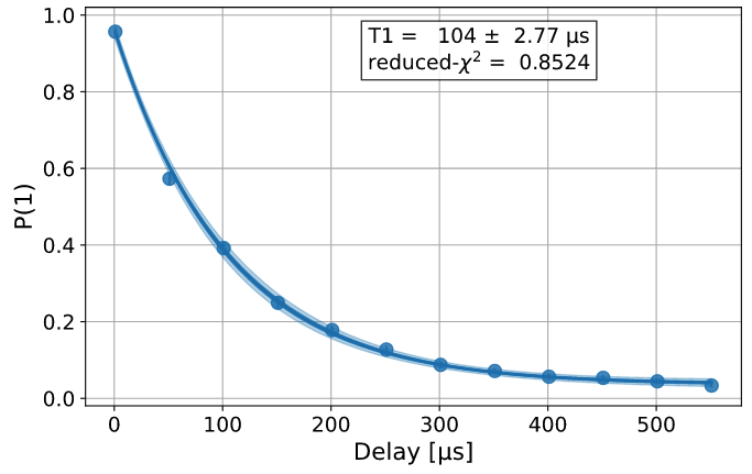
The analysis results have been retrieved as well:
for result in load_expdata.analysis_results():
    print(result)
AnalysisResult
- name: T1
- value: 0.0001040+/-0.0000028
- χ²: 0.8523786276663019
- quality: good
- extra: <1 items>
- device_components: ['Q0']
- verified: False
AnalysisResult
- name: @Parameters_T1Analysis
- value: CurveFitResult:
- fitting method: least_squares
- number of sub-models: 1
* F_exp_decay(x) = amp * exp(-x/tau) + base
- success: True
- number of function evals: 9
- degree of freedom: 9
- chi-square: 7.671407648996717
- reduced chi-square: 0.8523786276663019
- Akaike info crit.: 0.6311217041870707
- Bayesian info crit.: 2.085841653551072
- init params:
* amp = 0.923076923076923
* tau = 0.00016946294665316433
* base = 0.033466533466533464
- fit params:
* amp = 0.9266620487665083 ± 0.007096409569790425
* tau = 0.00010401411623191737 ± 2.767679521974391e-06
* base = 0.036302726197354626 ± 0.0037184540724124844
- correlations:
* (tau, base) = -0.6740808746060173
* (amp, base) = -0.4231810882291163
* (amp, tau) = 0.09302612202500576
- quality: good
- device_components: ['Q0']
- verified: False
Discussion#
Note that calling save() before the experiment is complete will
instantiate an experiment entry in the database, but it will not have
complete data. To fix this, you can call save() again once the
experiment is done running.
Sometimes the metadata of an experiment can be very large and cannot be stored directly in the database.
In this case, a separate metadata.json file will be stored along with the experiment. Saving and loading
this file is done automatically in save() and load().
Auto-saving an experiment#
The auto_save() feature automatically saves changes to the
ExperimentData object to the cloud service whenever it’s updated.
exp = T1(physical_qubits=(0,), delays=t1_delays)

t1_expdata = exp.run(backend=backend, shots=1000)
t1_expdata.auto_save = True
t1_expdata.block_for_results()
You can view the experiment online at https://quantum.ibm.com/experiments/cdaff3fa-f621-4915-a4d8-812d05d9a9ca
<ExperimentData[T1], backend: ibm_osaka, status: ExperimentStatus.DONE, experiment_id: cdaff3fa-f621-4915-a4d8-812d05d9a9ca>
Setting auto_save = True works by triggering ExperimentData.save().
When working with composite experiments, setting auto_save will propagate this
setting to the child experiments.
Deleting an experiment#
Both figures and analysis results can be deleted. Note that unless you
have auto save on, the update has to be manually saved to the remote
database by calling save(). Because there are two analysis
results, one for the T1 parameter and one for the curve fitting results, we must
delete twice to fully remove the analysis results.
t1_expdata.delete_figure(0)
t1_expdata.delete_analysis_result(0)
t1_expdata.delete_analysis_result(0)
Are you sure you want to delete the experiment plot? [y/N]: y
Are you sure you want to delete the analysis result? [y/N]: y
Are you sure you want to delete the analysis result? [y/N]: y
Tagging and sharing experiments#
Tags and notes can be added to experiments to help identify specific experiments in the interface. For example, an experiment can be tagged and made public with the following code.
t1_expdata.tags = ['tag1', 'tag2']
t1_expdata.share_level = "public"
t1_expdata.notes = "Example note."
Web interface#
You can also view experiment results as well as change the tags and share level at the IBM Quantum Experiments pane on the cloud.