Note
இந்தப் பக்கம் docs/tutorials/10_effective_dimension.ipynb. லிருந்து உருவாக்கப்பட்டது.
கிஸ்கிட் நரம்பியல் நெட்வொர்க்குகளின் பயனுள்ள பரிமாணம்#
இந்த டுடோரியலில், நாம் பயன்படுத்திக்கொள்வோம் EffectiveDimension மற்றும்``LocalEffectiveDimension`` வகுப்பு குவாண்டம் நியூரல் நெட்வொர்க் மாதிரிகளின் சக்தியை மதிப்பிடுவதற்கு. இவை தகவல் வடிவவியலின் அடிப்படையிலான அளவீடுகள் ஆகும், அவை பயிற்சி, வெளிப்படுத்துதல் அல்லது பொதுமைப்படுத்தும் திறன் போன்ற கருத்துகளுடன் இணைக்கப்படுகின்றன.
குறியீட்டு எடுத்துக்காட்டில் நுழைவதற்கு முன், இந்த இரண்டு அளவீடுகளுக்கும் இடையே உள்ள வித்தியாசம் என்ன என்பதையும், குவாண்டம் நியூரல் நெட்வொர்க்குகளின் ஆய்வுக்கு அவை ஏன் பொருத்தமானவை என்பதையும் சுருக்கமாக விளக்குவோம். உலகளாவிய பயனுள்ள பரிமாணத்தைப் பற்றிய கூடுதல் தகவல்களைக் காணலாம் this paper, உள்ளூர் பயனுள்ள பரிமாணம் அறிமுகப்படுத்தப்பட்டது later work.
1. Global vs. Local Effective Dimension#
Both classical and quantum machine learning models share a common goal: being good at generalizing, i.e. learning insights from data and applying them on unseen data.
இந்தத் திறனை மதிப்பிடுவதற்கு ஒரு நல்ல அளவீட்டைக் கண்டறிவது என்பது அற்பமான விஷயம் அல்ல. தி பவர் ஆஃப் குவாண்டம் நியூரல் நெட்வொர்க்குகளில், ஒரு குறிப்பிட்ட மாதிரியானது புதிய தரவுகளில் எவ்வளவு சிறப்பாகச் செயல்பட முடியும் என்பதற்கான பயனுள்ள குறிகாட்டியாக ஆசிரியர்கள் உலகளாவிய பயனுள்ள பரிமாணத்தை அறிமுகப்படுத்துகின்றனர். இயந்திர கற்றல் மாதிரிகளின் பயனுள்ள பரிமாணத்தில், இயந்திர கற்றல் மாதிரிகளின் பொதுமைப்படுத்தல் பிழையை கட்டுப்படுத்தும் புதிய திறன் அளவீடாக உள்ளூர் பயனுள்ள பரிமாணம் முன்மொழியப்பட்டது.
உலகளாவிய (எஃபெக்டிவ் டைமன்ஷன் வகுப்பு) மற்றும் உள்ளூர் பயனுள்ள பரிமாணம் (லோக்கல் எஃபெக்டிவ் டைமன்ஷன் வகுப்பு) ஆகியவற்றுக்கு இடையேயான முக்கிய வேறுபாடு உண்மையில் அவை கணக்கிடப்படும் விதத்தில் இல்லை, ஆனால் பகுப்பாய்வு செய்யப்படும் அளவுரு இடத்தின் தன்மையில் உள்ளது.. உலகளாவிய பயனுள்ள பரிமாணம் மாதிரியின் முழு அளவுரு இடத்தை ஒருங்கிணைக்கிறது, மேலும் பெரிய எண்ணிக்கையிலான அளவுரு (எடை) தொகுப்புகளிலிருந்து கணக்கிடப்படுகிறது. மறுபுறம், உள்ளூர் பயனுள்ள பரிமாணம், பயிற்சி பெற்ற மாதிரியானது புதிய தரவுகளுக்கு எவ்வளவு நன்றாகப் பொதுமைப்படுத்த முடியும், மேலும் அது எவ்வாறு வெளிப்படையாக இருக்கும் என்பதில் கவனம் செலுத்துகிறது. எனவே, உள்ளூர் பயனுள்ள பரிமாணம் ஒரே எடை மாதிரிகளின் தொகுப்பிலிருந்து கணக்கிடப்படுகிறது (பயிற்சி முடிவு). நடைமுறைச் செயலாக்கத்தின் அடிப்படையில் இந்த வேறுபாடு சிறியது, ஆனால் கருத்தியல் மட்டத்தில் மிகவும் பொருத்தமானது.
2. தி எஃபெக்டிவ் டைமன்ஷன் அல்காரிதம்#
Both the global and local effective dimension algorithms use the Fisher Information matrix to provide a measure of complexity. The details on how this matrix is calculated are provided in the reference paper, but in general terms, this matrix captures how sensitive a neural network’s output is to changes in the network’s parameter space.
குறிப்பாக, இந்த அல்காரிதம் 4 முக்கிய படிகளைப் பின்பற்றுகிறது:
மான்டே கார்லோ உருவகப்படுத்துதல்: ஒவ்வொரு ஜோடி உள்ளீடு மற்றும் எடை மாதிரிகளுக்கும் நரம்பியல் வலையமைப்பின் முன்னோக்கி மற்றும் பின்தங்கிய பாஸ்கள் (சாய்வுகள்) கணக்கிடப்படுகின்றன.
ஃபிஷர் மேட்ரிக்ஸ் கணக்கீடு: இந்த வெளியீடுகளும் சாய்வுகளும் ஃபிஷர் தகவல் மேட்ரிக்ஸைக் கணக்கிடப் பயன்படுத்தப்படுகின்றன.
ஃபிஷர் மேட்ரிக்ஸ் இயல்பாக்கம்: அனைத்து உள்ளீட்டு மாதிரிகளின் சராசரி மற்றும் மேட்ரிக்ஸ் ட்ரேஸ் மூலம் வகுத்தல்
பயனுள்ள பரிமாணக் கணக்கீடு: அப்பாஸ் மற்றும் பலர் வழங்கிய சூத்திரத்தின்படி.
3. Basic Example (SamplerQNN)#
This example shows how to set up a QNN model problem and run the global effective dimension algorithm. Both Qiskit SamplerQNN (shown in this example) and EstimatorQNN (shown in a later example) can be used with the EffectiveDimension class.
தேவையான இறக்குமதிகள் மற்றும் மறுஉற்பத்தி நோக்கங்களுக்காக சீரற்ற எண் ஜெனரேட்டருக்கான நிலையான விதையிலிருந்து தொடங்குகிறோம்.
[1]:
# Necessary imports
import matplotlib.pyplot as plt
import numpy as np
from IPython.display import clear_output
from qiskit import QuantumCircuit
from qiskit.circuit.library import ZFeatureMap, RealAmplitudes
from qiskit_algorithms.optimizers import COBYLA
from qiskit_algorithms.utils import algorithm_globals
from sklearn.datasets import make_classification
from sklearn.preprocessing import MinMaxScaler

from qiskit_machine_learning.circuit.library import QNNCircuit
from qiskit_machine_learning.algorithms.classifiers import NeuralNetworkClassifier
from qiskit_machine_learning.neural_networks import EffectiveDimension, LocalEffectiveDimension
from qiskit_machine_learning.neural_networks import SamplerQNN, EstimatorQNN

# set random seed
algorithm_globals.random_seed = 42
3.1 QNN ஐ வரையறுக்கவும்#
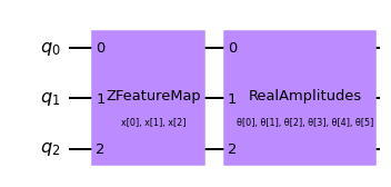
The first step to create a SamplerQNN is to define a parametrized feature map and ansatz. In this toy example, we will use 3 qubits and the QNNCircuit class to simplify the composition of a feature map and an ansatz circuit. The resulting circuit is then used in the SamplerQNN class.
[2]:
num_qubits = 3
# combine a custom feature map and ansatz into a single circuit
qc = QNNCircuit(
    feature_map=ZFeatureMap(feature_dimension=num_qubits, reps=1),
    ansatz=RealAmplitudes(num_qubits, reps=1),
)
qc.draw("mpl")
[2]:
The parametrized circuit can then be sent together with an optional interpret map (parity in this case) to the SamplerQNN constructor.
[3]:
# parity maps bitstrings to 0 or 1
def parity(x):
    return "{:b}".format(x).count("1") % 2


output_shape = 2  # corresponds to the number of classes, possible outcomes of the (parity) mapping.
[4]:
# construct QNN
qnn = SamplerQNN(
    circuit=qc,
    interpret=parity,
    output_shape=output_shape,
    sparse=False,
)
3.2 பயனுள்ள பரிமாண கணக்கீட்டை அமைக்கவும்#
EffectiveDimension வகுப்பைப் பயன்படுத்தி எங்கள் QNN இன் பயனுள்ள பரிமாணத்தைக் கணக்கிடுவதற்கு, உள்ளீட்டு மாதிரிகள் மற்றும் எடைகளின் தொடர் தொகுப்புகள் மற்றும் தரவுத்தொகுப்பில் கிடைக்கும் தரவு மாதிரிகளின் மொத்த எண்ணிக்கையும் தேவை. input_samples மற்றும் weight_samples ஆகியவை வகுப்பு கட்டமைப்பாளரில் அமைக்கப்பட்டுள்ளன, அதே நேரத்தில் பயனுள்ள பரிமாணக் கணக்கீட்டிற்கான அழைப்பின் போது தரவு மாதிரிகளின் எண்ணிக்கை வழங்கப்படுகிறது, இந்த அளவீடு வெவ்வேறு தரவுத்தொகுப்புடன் எவ்வாறு மாறுகிறது என்பதைச் சோதித்து ஒப்பிட்டுப் பார்க்க முடியும். அளவுகள்.
உள்ளீட்டு மாதிரிகள் மற்றும் எடை மாதிரிகளின் எண்ணிக்கையை நாம் வரையறுக்கலாம் மற்றும் வகுப்பு தோராயமாக ஒரு சாதாரண (input_samples) அல்லது ஒரு சீரான (weight_samples) விநியோகத்திலிருந்து தொடர்புடைய வரிசையை மாதிரி செய்யும். பல மாதிரிகளை அனுப்புவதற்குப் பதிலாக, ஒரு வரிசையை கைமுறையாக மாதிரியாக அனுப்பலாம்.
[5]:
# we can set the total number of input samples and weight samples for random selection
num_input_samples = 10
num_weight_samples = 10

global_ed = EffectiveDimension(
    qnn=qnn, weight_samples=num_weight_samples, input_samples=num_input_samples
)
உள்ளீட்டு மாதிரிகள் மற்றும் எடை மாதிரிகளின் குறிப்பிட்ட தொகுப்பைச் சோதிக்க விரும்பினால், பின்வரும் துணுக்கில் காட்டப்பட்டுள்ளபடி நேரடியாக EffectiveDimension வகுப்பிற்கு வழங்கலாம்:
[6]:
# we can also provide user-defined samples and parameters
input_samples = algorithm_globals.random.normal(0, 1, size=(10, qnn.num_inputs))
weight_samples = algorithm_globals.random.uniform(0, 1, size=(10, qnn.num_weights))

global_ed = EffectiveDimension(qnn=qnn, weight_samples=weight_samples, input_samples=input_samples)
பயனுள்ள பரிமாண அல்காரிதத்திற்கு தரவுத்தொகுப்பு அளவும் தேவைப்படுகிறது. இந்த எடுத்துக்காட்டில், இந்த உள்ளீடு முடிவை எவ்வாறு பாதிக்கிறது என்பதைப் பார்க்க, அளவுகளின் வரிசையை வரையறுப்போம்.
[7]:
# finally, we will define ranges to test different numbers of data, n
n = [5000, 8000, 10000, 40000, 60000, 100000, 150000, 200000, 500000, 1000000]
3.3 உலகளாவிய பயனுள்ள பரிமாணத்தைக் கணக்கிடுங்கள்#
Let’s now calculate the effective dimension of our network for the previously defined set of input samples, weights, and a dataset size of 5000.
[8]:
global_eff_dim_0 = global_ed.get_effective_dimension(dataset_size=n[0])
The effective dimension values will range between 0 and d, where d represents the dimension of the model, and it’s practically obtained from the number of weights of the QNN. By dividing the result by d, we can obtain the normalized effective dimension, which correlates directly with the capacity of the model.
[9]:
d = qnn.num_weights

print("Data size: {}, global effective dimension: {:.4f}".format(n[0], global_eff_dim_0))
print(
    "Number of weights: {}, normalized effective dimension: {:.4f}".format(d, global_eff_dim_0 / d)
)
Data size: 5000, global effective dimension: 4.6657
Number of weights: 6, normalized effective dimension: 0.7776
உள்ளீட்டு அளவுகள் n எனில் அணிவரிசையுடன் EffectiveDimension வகுப்பை அழைப்பதன் மூலம், தரவுத்தொகுப்பின் அளவுடன் பயனுள்ள பரிமாணம் எவ்வாறு மாறுகிறது என்பதைக் கண்காணிக்கலாம்.
[10]:
global_eff_dim_1 = global_ed.get_effective_dimension(dataset_size=n)
[11]:
print("Effective dimension: {}".format(global_eff_dim_1))
print("Number of weights: {}".format(d))
Effective dimension: [4.66565096 4.7133723  4.73782922 4.89963559 4.94632272 5.00280009
 5.04530433 5.07408394 5.15786005 5.21349874]
Number of weights: 6
[12]:
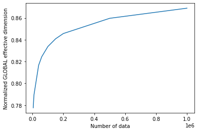
# plot the normalized effective dimension for the model
plt.plot(n, np.array(global_eff_dim_1) / d)
plt.xlabel("Number of data")
plt.ylabel("Normalized GLOBAL effective dimension")
plt.show()
4. லோக்கல் எஃபெக்டிவ் டைமன்ஷன் உதாரணம்#
அறிமுகத்தில் விளக்கப்பட்டுள்ளபடி, உள்ளூர் பயனுள்ள பரிமாண வழிமுறையானது ஒன்று எடைகளின் தொகுப்பை மட்டுமே பயன்படுத்துகிறது, மேலும் பயிற்சியானது நரம்பியல் வலையமைப்பின் வெளிப்பாட்டை எவ்வாறு பாதிக்கிறது என்பதைக் கண்காணிக்கப் பயன்படுகிறது. இந்தக் கணக்கீடுகள் கருத்தியல் ரீதியாக தனித்தனியாக இருப்பதை உறுதிசெய்ய LocalEffective Dimension வகுப்பு இந்தக் கட்டுப்பாட்டைச் செயல்படுத்துகிறது, ஆனால் மீதமுள்ள செயல்படுத்தல் Effective Dimension உடன் பகிரப்படுகிறது.
QNN வெளிப்பாட்டின் மீதான பயிற்சியின் விளைவை பகுப்பாய்வு செய்ய LocalEffective Dimension வகுப்பை எவ்வாறு பயன்படுத்துவது என்பதை இந்த எடுத்துக்காட்டு காட்டுகிறது.
4.1 தரவுத்தொகுப்பு மற்றும் QNN ஐ வரையறுக்கவும்#
We start by creating a 3D binary classification dataset using make_classification function from scikit-learn.
[13]:
num_inputs = 3
num_samples = 50

X, y = make_classification(
    n_samples=num_samples,
    n_features=num_inputs,
    n_informative=3,
    n_redundant=0,
    n_clusters_per_class=1,
    class_sep=2.0,
)
X = MinMaxScaler().fit_transform(X)
y = 2 * y - 1  # labels in {-1, 1}
The next step is to create a QNN, an instance of EstimatorQNN in our case in the same fashion we created an instance of SamplerQNN.
[14]:
estimator_qnn = EstimatorQNN(circuit=qc)
4.2 ரயில் QNN#
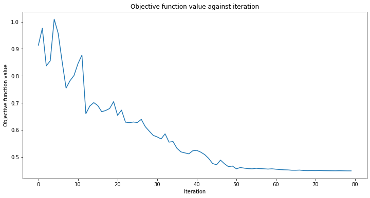
நாம் இப்போது QNN க்கு பயிற்சி அளிக்கத் தொடரலாம். பயிற்சி படி சிறிது நேரம் ஆகலாம், பொறுமையாக இருங்கள். பயிற்சி செயல்முறை எவ்வாறு நடக்கிறது என்பதைக் கவனிக்க, வகைப்படுத்திக்கு நீங்கள் திரும்ப அழைப்பை அனுப்பலாம். வழக்கம்போல் மறுஉருவாக்கம் நோக்கங்களுக்காக initial_point ஐ சரிசெய்கிறோம்.
[15]:
# callback function that draws a live plot when the .fit() method is called
def callback_graph(weights, obj_func_eval):
    clear_output(wait=True)
    objective_func_vals.append(obj_func_eval)
    plt.title("Objective function value against iteration")
    plt.xlabel("Iteration")
    plt.ylabel("Objective function value")
    plt.plot(range(len(objective_func_vals)), objective_func_vals)
    plt.show()
[16]:
# construct classifier
initial_point = algorithm_globals.random.random(estimator_qnn.num_weights)

estimator_classifier = NeuralNetworkClassifier(
    neural_network=estimator_qnn,
    optimizer=COBYLA(maxiter=80),
    initial_point=initial_point,
    callback=callback_graph,
)
[17]:
# create empty array for callback to store evaluations of the objective function (callback)
objective_func_vals = []
plt.rcParams["figure.figsize"] = (12, 6)

# fit classifier to data
estimator_classifier.fit(X, y)

# return to default figsize
plt.rcParams["figure.figsize"] = (6, 4)
வகைப்படுத்தி இப்போது வகுப்புகளை துல்லியமாக வேறுபடுத்த முடியும்:
[18]:
# score classifier
estimator_classifier.score(X, y)
[18]:
0.96
4.3 பயிற்சியளிக்கப்பட்ட QNN இன் உள்ளூர் பயனுள்ள பரிமாணத்தைக் கணக்கிடுங்கள்#
Now that we have trained our network, let’s evaluate the local effective dimension based on the trained weights. To do that we access the trained weights directly from the classifier.
[19]:
trained_weights = estimator_classifier.weights

# get Local Effective Dimension for set of trained weights
local_ed_trained = LocalEffectiveDimension(
    qnn=estimator_qnn, weight_samples=trained_weights, input_samples=X
)

local_eff_dim_trained = local_ed_trained.get_effective_dimension(dataset_size=n)

print(
    "normalized local effective dimensions for trained QNN: ",
    local_eff_dim_trained / estimator_qnn.num_weights,
)
normalized local effective dimensions for trained QNN:  [0.38001027 0.38667693 0.39017714 0.41507888 0.42307677 0.43341398
 0.44170977 0.44758111 0.46577231 0.4786767 ]
4.4 பயிற்சி பெறாத QNN இன் உள்ளூர் பயனுள்ள பரிமாணத்தைக் கணக்கிடுங்கள்#
எங்கள் எடை மாதிரியாக initial_point ஐப் பயன்படுத்தி, பயிற்சி பெறாத நெட்வொர்க்கின் பயனுள்ள பரிமாணத்துடன் இந்த முடிவை ஒப்பிடலாம்:
[20]:
# get Local Effective Dimension for set of untrained weights
local_ed_untrained = LocalEffectiveDimension(
    qnn=estimator_qnn, weight_samples=initial_point, input_samples=X
)

local_eff_dim_untrained = local_ed_untrained.get_effective_dimension(dataset_size=n)

print(
    "normalized local effective dimensions for untrained QNN: ",
    local_eff_dim_untrained / estimator_qnn.num_weights,
)
normalized local effective dimensions for untrained QNN:  [0.69803061 0.7130991  0.7203237  0.76321615 0.77452215 0.7877625
 0.79746712 0.8039319  0.82236146 0.83435907]
4.5 முடிவுகளை வரைந்து பகுப்பாய்வு செய்யுங்கள்#
பயிற்சிக்கு முன்னும் பின்னும் பயனுள்ள பரிமாண மதிப்புகளை நாம் திட்டமிட்டால், பின்வரும் முடிவைக் காணலாம்:
[21]:
# plot the normalized effective dimension for the model
plt.plot(n, np.array(local_eff_dim_trained) / estimator_qnn.num_weights, label="trained weights")
plt.plot(
    n, np.array(local_eff_dim_untrained) / estimator_qnn.num_weights, label="untrained weights"
)

plt.xlabel("Number of data")
plt.ylabel("Normalized LOCAL effective dimension")
plt.legend()
plt.show()
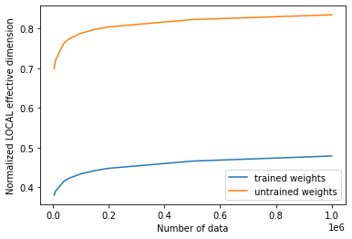
பொதுவாக, பயிற்சிக்குப் பிறகு உள்ளூர் பயனுள்ள பரிமாணத்தின் மதிப்பு குறையும் என்று எதிர்பார்க்க வேண்டும். மெஷின் லேர்னிங்கின் முக்கிய இலக்கைத் திரும்பிப் பார்ப்பதன் மூலம் இதைப் புரிந்து கொள்ள முடியும், இது உங்கள் தரவுகளுக்குப் பொருந்தக்கூடிய அளவுக்கு வெளிப்படுத்தக்கூடிய மாதிரியைத் தேர்ந்தெடுப்பது, ஆனால் புதிய தரவு மாதிரிகளில் மிகையாகப் பொருந்தி மோசமாகச் செயல்படும் மாதிரியைத் தேர்ந்தெடுப்பது அல்ல.
கற்றல் அளவுருக்கள் மூலம் ஒரு மாதிரியின் அதிகப்படியான பொருத்தத்தை முறைப்படுத்த சில உகப்பாக்கிகள் உதவுகின்றன, மேலும் இந்த கற்றல் செயல், உள்ளூர் பயனுள்ள பரிமாணத்தால் அளவிடப்படும் மாதிரியின் வெளிப்பாட்டுத்தன்மையை இயல்பாகவே குறைக்கிறது. இந்த தர்க்கத்தைப் பின்பற்றி, தோராயமாக துவக்கப்பட்ட அளவுரு தொகுப்பு, பயிற்சி பெற்ற எடைகளின் இறுதித் தொகுப்பை விட அதிக செயல்திறன் கொண்ட பரிமாணத்தை உருவாக்கும், ஏனெனில் அந்த குறிப்பிட்ட அளவுருவுடன் கூடிய அந்த மாதிரியானது தரவை பொருத்துவதற்கு தேவையில்லாமல் "அதிக அளவுருக்களைப் பயன்படுத்துகிறது". பயிற்சிக்குப் பிறகு (மறைமுகமான முறைப்படுத்தலுடன்), பயிற்சியளிக்கப்பட்ட மாதிரி பல அளவுருக்களைப் பயன்படுத்த வேண்டிய அவசியமில்லை, இதனால் அதிக "செயலற்ற அளவுருக்கள்" மற்றும் குறைந்த செயல்திறன் பரிமாணம் இருக்கும்.
We must keep in mind though that this is the general intuition, and there might be cases where a randomly selected set of weights happens to provide a lower effective dimension than the trained weights for a specific model.
[22]:
import qiskit.tools.jupyter

%qiskit_version_table
%qiskit_copyright
Version Information
| Qiskit Software | Version |
|---|---|
qiskit-terra | 0.24.0 |
qiskit-aer | 0.12.0 |
qiskit-ignis | 0.6.0 |
qiskit-ibmq-provider | 0.20.2 |
qiskit | 0.43.0 |
qiskit-machine-learning | 0.7.0 |
| System information | |
| Python version | 3.8.8 |
| Python compiler | Clang 10.0.0 |
| Python build | default, Apr 13 2021 12:59:45 |
| OS | Darwin |
| CPUs | 8 |
| Memory (Gb) | 32.0 |
| Tue Jun 13 16:40:08 2023 CEST | |
This code is a part of Qiskit
© Copyright IBM 2017, 2023.
This code is licensed under the Apache License, Version 2.0. You may
obtain a copy of this license in the LICENSE.txt file in the root directory
of this source tree or at http://www.apache.org/licenses/LICENSE-2.0.
Any modifications or derivative works of this code must retain this
copyright notice, and modified files need to carry a notice indicating
that they have been altered from the originals.