Note

இந்தப் பக்கம் docs/tutorials/02a_training_a_quantum_model_on_a_real_dataset.ipynb இலிருந்து உருவாக்கப்பட்டது.

உண்மையான தரவுத்தொகுப்பில் குவாண்டம் மாதிரியைப் பயிற்றுவித்தல்

வகைப்பாடு சிக்கலைச் சமாளிக்க குவாண்டம் இயந்திர கற்றல் மாதிரியை எவ்வாறு பயிற்றுவிப்பது என்பதை இந்தப் பயிற்சி விளக்குகிறது. முந்தைய பயிற்சிகள் சிறிய, செயற்கை தரவுத்தொகுப்புகளைக் கொண்டிருந்தன. இங்கே நிஜ வாழ்க்கை கிளாசிக்கல் தரவுத்தொகுப்பைக் கருத்தில் கொண்டு சிக்கலின் சிக்கலை அதிகரிப்போம். மிகவும் நன்கு அறியப்பட்ட - இன்னும் சிறியதாக இருந்தாலும் - பிரச்சனை: ஐரிஸ் மலர் தரவுத்தொகுப்பைத் தேர்வுசெய்ய முடிவு செய்தோம். இந்தத் தரவுத்தொகுப்பில் அதன் சொந்த விக்கிபீடியா பக்கம் உள்ளது. ஐரிஸ் தரவுத்தொகுப்பு தரவு விஞ்ஞானிகளுக்கு நன்கு தெரிந்திருந்தாலும், நமது நினைவுகளைப் புதுப்பிக்க சுருக்கமாக அதை அறிமுகப்படுத்துவோம். ஒப்பிடுகையில், முதலில் குவாண்டம் மாதிரிக்கு ஒரு கிளாசிக்கல் ஒப்பீட்டைப் பயிற்றுவிப்போம்.

எனவே, தொடங்குவோம்:

• First, we’ll load the dataset and explore what it looks like.

• Next, we’ll train a classical model using SVC from scikit-learn to see how well the classification problem can be solved using classical methods.

• அதன் பிறகு, நாம் விரிவான Quantum Classifier (VQC) அறிமுகம் செய்யும்.

• முடிவுக்கு, நாங்கள் இரண்டு மாதிரிகளில் இருந்து பெறப்பட்ட முடிவுகளையும் ஒப்பிடுவேன்.

1. ஆய்வுத் தரவுப் பகுப்பாய்வு

முதலில், இந்த டுடோரியல் பயன்படுத்தும் ஐரிஸ் தரவுத்தொகுப்பை ஆராய்ந்து அதில் என்ன இருக்கிறது என்பதைப் பார்ப்போம். எங்கள் வசதிக்காக, இந்த டேட்டாசெட் scikit-learnல் கிடைக்கிறது மற்றும் எளிதாக ஏற்ற முடியும்.

from sklearn.datasets import load_iris

iris_data = load_iris()

If no parameters are specified in the load_iris function, then a dictionary-like object is returned by scikit-learn. Let’s print the description of the dataset and see what is inside.

print(iris_data.DESCR)

.. _iris_dataset:

Iris plants dataset
--------------------

**Data Set Characteristics:**

    :Number of Instances: 150 (50 in each of three classes)
    :Number of Attributes: 4 numeric, predictive attributes and the class
    :Attribute Information:
        - sepal length in cm
        - sepal width in cm
        - petal length in cm
        - petal width in cm
        - class:
                - Iris-Setosa
                - Iris-Versicolour
                - Iris-Virginica

    :Summary Statistics:

    ============== ==== ==== ======= ===== ====================
                    Min  Max   Mean    SD   Class Correlation
    ============== ==== ==== ======= ===== ====================
    sepal length:   4.3  7.9   5.84   0.83    0.7826
    sepal width:    2.0  4.4   3.05   0.43   -0.4194
    petal length:   1.0  6.9   3.76   1.76    0.9490  (high!)
    petal width:    0.1  2.5   1.20   0.76    0.9565  (high!)
    ============== ==== ==== ======= ===== ====================

    :Missing Attribute Values: None
    :Class Distribution: 33.3% for each of 3 classes.
    :Creator: R.A. Fisher
    :Donor: Michael Marshall (MARSHALL%PLU@io.arc.nasa.gov)
    :Date: July, 1988

The famous Iris database, first used by Sir R.A. Fisher. The dataset is taken
from Fisher's paper. Note that it's the same as in R, but not as in the UCI
Machine Learning Repository, which has two wrong data points.

This is perhaps the best known database to be found in the
pattern recognition literature.  Fisher's paper is a classic in the field and
is referenced frequently to this day.  (See Duda & Hart, for example.)  The
data set contains 3 classes of 50 instances each, where each class refers to a
type of iris plant.  One class is linearly separable from the other 2; the
latter are NOT linearly separable from each other.

.. topic:: References

   - Fisher, R.A. "The use of multiple measurements in taxonomic problems"
     Annual Eugenics, 7, Part II, 179-188 (1936); also in "Contributions to
     Mathematical Statistics" (John Wiley, NY, 1950).
   - Duda, R.O., & Hart, P.E. (1973) Pattern Classification and Scene Analysis.
     (Q327.D83) John Wiley & Sons.  ISBN 0-471-22361-1.  See page 218.
   - Dasarathy, B.V. (1980) "Nosing Around the Neighborhood: A New System
     Structure and Classification Rule for Recognition in Partially Exposed
     Environments".  IEEE Transactions on Pattern Analysis and Machine
     Intelligence, Vol. PAMI-2, No. 1, 67-71.
   - Gates, G.W. (1972) "The Reduced Nearest Neighbor Rule".  IEEE Transactions
     on Information Theory, May 1972, 431-433.
   - See also: 1988 MLC Proceedings, 54-64.  Cheeseman et al"s AUTOCLASS II
     conceptual clustering system finds 3 classes in the data.
   - Many, many more ...

இந்தத் தரவுத்தொகுப்பு விளக்கத்திலிருந்து நாம் காணக்கூடிய சில சுவாரஸ்யமான அவதானிப்புகள் உள்ளன:

• தரவுத்தொகுப்பில் 150 மாதிரிகள் (நிகழ்வுகள்) உள்ளன.

• ஒவ்வொரு மாதிரியிலும் நான்கு அம்சங்கள் (பண்புகள்) உள்ளன.

• தரவுத்தொகுப்பில் மூன்று லேபிள்கள் (வகுப்புகள்) உள்ளன.

• ஒவ்வொரு வகுப்பிலும் ஒரே மாதிரியான மாதிரிகள் (50) இருப்பதால், தரவுத்தொகுப்பு முற்றிலும் சமநிலையில் உள்ளது.

• அம்சங்கள் இயல்பாக்கப்படாமல் இருப்பதையும், அவற்றின் மதிப்பு வரம்புகள் வேறுபட்டிருப்பதையும் பார்க்கலாம், எ.கா., \([4.3, 7.9]\) மற்றும் \([0.1, 2.5]\) முறையே செப்பல் நீளம் மற்றும் இதழ் அகலம். எனவே, அம்சங்களை ஒரே அளவில் மாற்றுவது உதவியாக இருக்கும்.

• மேலே உள்ள அட்டவணையில் கூறப்பட்டுள்ளபடி, சில சந்தர்ப்பங்களில் அம்சம்-வகுப்பு தொடர்பு மிகவும் அதிகமாக உள்ளது; இது எங்கள் மாதிரி தரவுத்தொகுப்பைச் சரியாகச் சமாளிக்க வேண்டும் என்று நினைக்க வழிவகுக்கும்.

தரவுத்தொகுப்பு விளக்கத்தை மட்டுமே நாங்கள் ஆய்வு செய்தோம், ஆனால் கூடுதல் பண்புகள் iris_data பொருளில் உள்ளன. இப்போது நாம் தரவுத்தொகுப்பிலிருந்து அம்சங்கள் மற்றும் லேபிள்களுடன் வேலை செய்யப் போகிறோம்.

features = iris_data.data
labels = iris_data.target

Firstly, we’ll normalize the features. Namely, we will apply a simple transformation to represent all features on the same scale. In our case, we squeeze all features onto the interval \([0, 1]\). Normalization is a common technique in machine learning and often leads to better numerical stability and convergence of an algorithm.

இதைச் செய்ய, scikit-learn இலிருந்து MinMaxScaler ஐப் பயன்படுத்தலாம். அளவுருக்களைக் குறிப்பிடாமல், இது சரியாகத் தேவையானதைச் செய்கிறது: \([0, 1]\) இல் தரவை வரைபடமாக்குகிறது.

from sklearn.preprocessing import MinMaxScaler

features = MinMaxScaler().fit_transform(features)

Let’s see how our data looks. We plot the features pair-wise to see if there’s an observable correlation between them.

import pandas as pd
import seaborn as sns

df = pd.DataFrame(iris_data.data, columns=iris_data.feature_names)
df["class"] = pd.Series(iris_data.target)

sns.pairplot(df, hue="class", palette="tab10")

<seaborn.axisgrid.PairGrid at 0x1c92dbc4188>

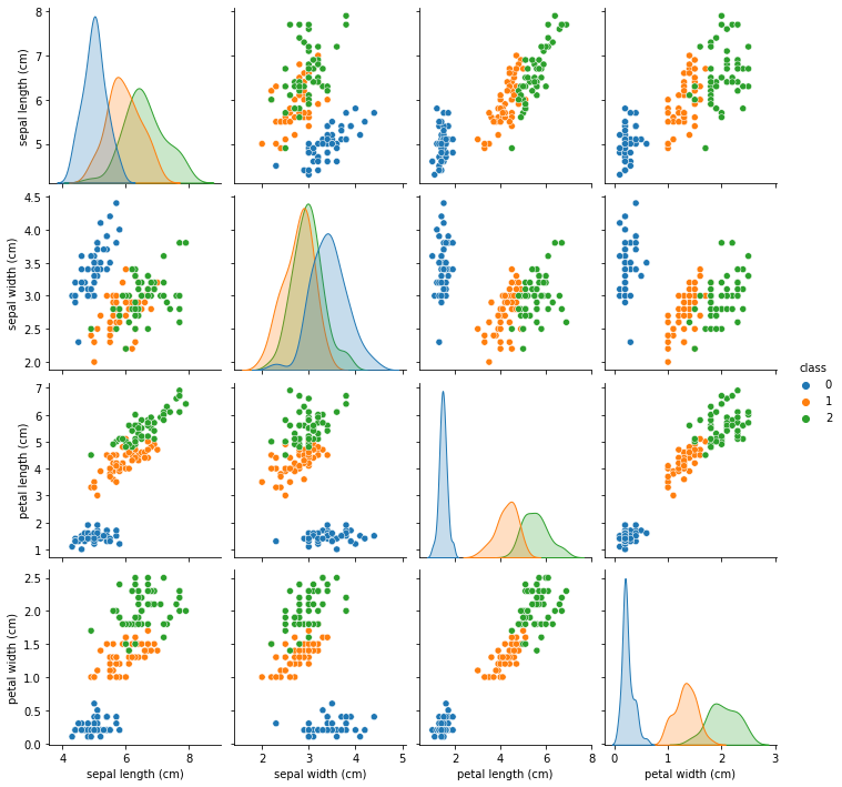
From the plots, we see that class 0 is easily separable from the other two classes, while classes 1 and 2 are sometimes intertwined, especially regarding the "sepal width" feature.

Next, let’s see how classical machine learning handles this dataset.

2. கிளாசிக்கல் மெஷின் கற்றல் மாதிரியைப் பயிற்றுவித்தல்

Before we train a model, we should split the dataset into two parts: a training dataset and a test dataset. We’ll use the former to train the model and the latter to verify how well our models perform on unseen data.

As usual, we’ll ask scikit-learn to do the boring job for us. We’ll also fix the seed to ensure the results are reproducible.

from sklearn.model_selection import train_test_split
from qiskit_algorithms.utils import algorithm_globals

algorithm_globals.random_seed = 123
train_features, test_features, train_labels, test_labels = train_test_split(
    features, labels, train_size=0.8, random_state=algorithm_globals.random_seed
)

We train a classical Support Vector Classifier from scikit-learn. For the sake of simplicity, we don’t tweak any parameters and rely on the default values.

from sklearn.svm import SVC

svc = SVC()
_ = svc.fit(train_features, train_labels)  # suppress printing the return value

எங்கள் கிளாசிக்கல் மாடல் எவ்வளவு சிறப்பாகச் செயல்படுகிறது என்பதை இப்போது பார்க்கிறோம். முடிவுப் பிரிவில் மதிப்பெண்களைப் பகுப்பாய்வு செய்வோம்.

train_score_c4 = svc.score(train_features, train_labels)
test_score_c4 = svc.score(test_features, test_labels)

print(f"Classical SVC on the training dataset: {train_score_c4:.2f}")
print(f"Classical SVC on the test dataset:     {test_score_c4:.2f}")

Classical SVC on the training dataset: 0.99
Classical SVC on the test dataset:     0.97

As can be seen from the scores, the classical SVC algorithm performs very well. Next up, it’s time to look at quantum machine learning models.

3. குவாண்டம் மெஷின் கற்றல் மாதிரியைப் பயிற்றுவித்தல்

ஒரு குவாண்டம் மாதிரியின் உதாரணமாக, ஒரு மாறுபாடு குவாண்டம் வகைப்படுத்தியை (VQC) பயிற்றுவிப்போம். VQC என்பது கிஸ்கிட் மெஷின் லேர்னிங்கில் கிடைக்கும் எளிமையான வகைப்படுத்தியாகும், மேலும் இது கிளாசிக்கல் மெஷின் லேர்னிங்கில் பின்னணியைக் கொண்ட குவாண்டம் மெஷின் லேர்னிங்கில் புதிதாக வருபவர்களுக்கு ஒரு நல்ல தொடக்கப் புள்ளியாகும்.

ஆனால் ஒரு மாதிரியைப் பயிற்றுவிப்பதற்கு முன், VQC வகுப்பை உள்ளடக்கியதாக ஆராய்வோம். அதன் இரண்டு மையக் கூறுகள் அம்ச வரைபடம் மற்றும் அன்சாட்ஸ் ஆகும். இவை என்ன என்பது இப்போது விளக்கப்படும்.

எங்கள் தரவு கிளாசிக்கல், அதாவது இது பிட்களின் தொகுப்பைக் கொண்டுள்ளது, குவிட்கள் அல்ல. தரவை குவிட்களாக குறியாக்கம் செய்ய நமக்கு ஒரு வழி தேவை. பயனுள்ள குவாண்டம் மாதிரியைப் பெற விரும்பினால் இந்த செயல்முறை முக்கியமானது. நாங்கள் வழக்கமாக இந்த மேப்பிங்கை தரவு குறியாக்கம், தரவு உட்பொதித்தல் அல்லது தரவு ஏற்றுதல் என குறிப்பிடுகிறோம், இதுவே அம்ச வரைபடத்தின் பங்கு. அம்ச மேப்பிங் ஒரு பொதுவான ML பொறிமுறையாக இருந்தாலும், குவாண்டம் நிலைகளில் தரவை ஏற்றும் இந்த செயல்முறை கிளாசிக்கல் இயந்திர கற்றலில் தோன்றாது, ஏனெனில் இது கிளாசிக்கல் உலகில் மட்டுமே செயல்படுகிறது.

தரவு ஏற்றப்பட்டதும், நாம் உடனடியாக ஒரு அளவுரு குவாண்டம் சர்க்யூட்டைப் பயன்படுத்த வேண்டும். இந்த சுற்று கிளாசிக்கல் நரம்பியல் நெட்வொர்க்குகளில் உள்ள அடுக்குகளுக்கு நேரடி அனலாக் ஆகும். இது சரிசெய்யக்கூடிய அளவுருக்கள் அல்லது எடைகளின் தொகுப்பைக் கொண்டுள்ளது. எடைகள் ஒரு புறநிலை செயல்பாட்டைக் குறைக்கும் வகையில் உகந்ததாக இருக்கும். இந்த புறநிலை செயல்பாடு கணிப்புகள் மற்றும் அறியப்பட்ட லேபிளிடப்பட்ட தரவுகளுக்கு இடையிலான தூரத்தை வகைப்படுத்துகிறது. ஒரு அளவுருவாக்கப்பட்ட குவாண்டம் சர்க்யூட் ஒரு அளவுருப்படுத்தப்பட்ட சோதனை நிலை, மாறுபாடு வடிவம் அல்லது அன்சாட்ஸ் என்றும் அழைக்கப்படுகிறது. ஒருவேளை, பிந்தையது மிகவும் பரவலாகப் பயன்படுத்தப்படும் சொல்.

For more information, we direct the reader to the Quantum Machine Learning Course.

அம்ச வரைபடத்தின் எங்கள் தேர்வு ZZFeatureMap ஆகும். ZZFeatureMap` என்பது Qiskit சர்க்யூட் லைப்ரரியில் உள்ள நிலையான அம்ச வரைபடங்களில் ஒன்றாகும். ``num_features என்பதை feature_dimension எனக் கடந்து செல்கிறோம், அதாவது அம்ச வரைபடத்தில் num_features அல்லது 4 குவிட்கள் இருக்கும்.

அம்ச வரைபடங்கள் எவ்வாறு தோற்றமளிக்கலாம் என்பதை வாசகருக்கு வழங்க, அம்ச வரைபடத்தை அதன் தொகுதி வாயில்களாகச் சிதைக்கிறோம்.

from qiskit.circuit.library import ZZFeatureMap

num_features = features.shape[1]

feature_map = ZZFeatureMap(feature_dimension=num_features, reps=1)
feature_map.decompose().draw(output="mpl", fold=20)

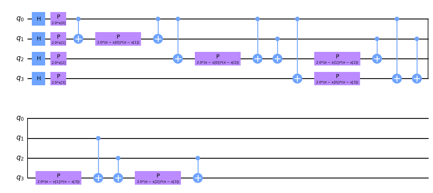
அம்ச வரைபட வரைபடத்தை நீங்கள் உற்று நோக்கினால், x[0], ..., x[3] அளவுருக்களைக் காண்பீர்கள். இவை எங்கள் அம்சங்களுக்கான ஒதுக்கிடங்கள்.

இப்போது நாங்கள் எங்கள் அன்சாட்ஸை உருவாக்கி, திட்டமிடுகிறோம். அன்சாட்ஸ் சுற்றுகளின் மீண்டும் மீண்டும் கட்டமைப்பிற்கு கவனம் செலுத்துங்கள். reps அளவுருவைப் பயன்படுத்தி இந்த மறுநிகழ்வுகளின் எண்ணிக்கையை நாங்கள் வரையறுக்கிறோம்.

from qiskit.circuit.library import RealAmplitudes

ansatz = RealAmplitudes(num_qubits=num_features, reps=3)
ansatz.decompose().draw(output="mpl", fold=20)

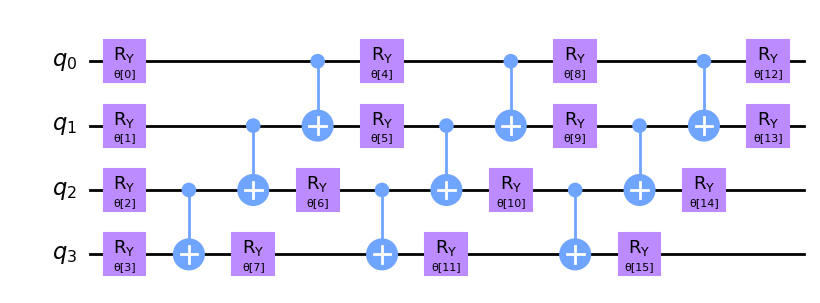
இந்தச் சுற்றுக்கு θ[0], ..., θ[15] என்ற 16 அளவுருக்கள் உள்ளன. இவை வகைப்படுத்தியின் பயிற்சிக்குரிய எடைகள்.

பயிற்சி செயல்பாட்டில் பயன்படுத்த ஒரு தேர்வுமுறை அல்காரிதத்தை நாங்கள் தேர்வு செய்கிறோம். கிளாசிக்கல் டீப் லேர்னிங் ஃப்ரேம்வொர்க்குகளில் நீங்கள் காணக்கூடியதைப் போலவே இந்தப் படியும் இருக்கும். பயிற்சி செயல்முறையை விரைவுபடுத்த, சாய்வு இல்லாத ஆப்டிமைசரை நாங்கள் தேர்வு செய்கிறோம். Qiskit இல் கிடைக்கும் பிற உகப்பாக்கிகளை நீங்கள் ஆராயலாம்.

from qiskit_algorithms.optimizers import COBYLA

optimizer = COBYLA(maxiter=100)

அடுத்த கட்டத்தில், எங்கள் வகைப்படுத்திக்கு எங்கு பயிற்சி அளிக்க வேண்டும் என்பதை நாங்கள் வரையறுக்கிறோம். நாம் ஒரு சிமுலேட்டர் அல்லது உண்மையான குவாண்டம் கணினியில் பயிற்சி பெறலாம். இங்கே, நாம் ஒரு சிமுலேட்டரைப் பயன்படுத்துவோம். Sampler பழமையான நிகழ்வை உருவாக்குகிறோம். இது ஸ்டேட்வெக்டர் அடிப்படையிலான குறிப்பு செயலாக்கமாகும். qiskit இயக்க நேர சேவைகளைப் பயன்படுத்தி, நீங்கள் ஒரு குவாண்டம் கணினியால் ஆதரிக்கப்படும் மாதிரியை உருவாக்கலாம்.

from qiskit.primitives import Sampler

sampler = Sampler()

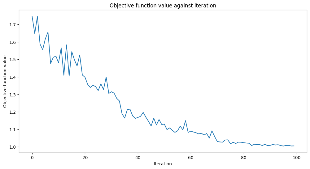
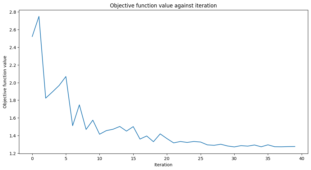
callback_graph என்றழைக்கப்படும் கால்பேக் செயல்பாட்டைச் சேர்ப்போம். புறநிலை செயல்பாட்டின் ஒவ்வொரு மதிப்பீட்டிற்கும் VQC இந்தச் செயல்பாட்டை இரண்டு அளவுருக்களுடன் அழைக்கும்: தற்போதைய எடைகள் மற்றும் அந்த எடைகளில் உள்ள புறநிலை செயல்பாட்டின் மதிப்பு. எங்கள் கால்பேக் புறநிலை செயல்பாட்டின் மதிப்பை ஒரு அணியில் சேர்க்கும், எனவே புறநிலை செயல்பாடு மதிப்புக்கு எதிராக மறு செய்கையை நாம் திட்டமிடலாம். அழைப்பு ஒவ்வொரு மறு செய்கையிலும் ப்ளாட்டை புதுப்பிக்கும். நாம் மேலே குறிப்பிட்டுள்ள இரண்டு அளவுரு கையொப்பம் இருக்கும் வரை, ஒரு கால்பேக் செயல்பாட்டிற்குள் நீங்கள் என்ன வேண்டுமானாலும் செய்யலாம் என்பதை நினைவில் கொள்ளவும்.

from matplotlib import pyplot as plt
from IPython.display import clear_output

objective_func_vals = []
plt.rcParams["figure.figsize"] = (12, 6)


def callback_graph(weights, obj_func_eval):
    clear_output(wait=True)
    objective_func_vals.append(obj_func_eval)
    plt.title("Objective function value against iteration")
    plt.xlabel("Iteration")
    plt.ylabel("Objective function value")
    plt.plot(range(len(objective_func_vals)), objective_func_vals)
    plt.show()

இப்போது நாங்கள் வகைப்படுத்தியை உருவாக்கி அதைப் பொருத்த தயாராக இருக்கிறோம்.

VQC` என்பது "மாறுபட்ட குவாண்டம் வகைப்படுத்தி" என்பதைக் குறிக்கிறது. இது ஒரு அம்ச வரைபடம் மற்றும் ஒரு அன்சாட்ஸை எடுத்து தானாகவே ஒரு குவாண்டம் நியூரல் நெட்வொர்க்கை உருவாக்குகிறது. எளிமையான வழக்கில், சரியான வகைப்படுத்தியை உருவாக்க, குவிட்களின் எண்ணிக்கையையும் குவாண்டம் நிகழ்வையும் அனுப்பினால் போதும். நீங்கள் ``மாதிரி அளவுருவைத் தவிர்க்கலாம், இந்தச் சந்தர்ப்பத்தில் நாங்கள் முன்பு உருவாக்கிய வழியில் உங்களுக்காக மாதிரி நிகழ்வு உருவாக்கப்படும். விளக்க நோக்கங்களுக்காக மட்டுமே நாங்கள் அதை கைமுறையாக உருவாக்கியுள்ளோம்.

பயிற்சி சிறிது நேரம் ஆகலாம். தயவுசெய்து பொறுமையாக இருங்கள்.

import time
from qiskit_machine_learning.algorithms.classifiers import VQC

vqc = VQC(
    sampler=sampler,
    feature_map=feature_map,
    ansatz=ansatz,
    optimizer=optimizer,
    callback=callback_graph,
)

# clear objective value history
objective_func_vals = []

start = time.time()
vqc.fit(train_features, train_labels)
elapsed = time.time() - start

print(f"Training time: {round(elapsed)} seconds")

Training time: 303 seconds

நிஜ வாழ்க்கை தரவுத்தொகுப்பில் குவாண்டம் மாதிரி எவ்வாறு செயல்படுகிறது என்பதைப் பார்ப்போம்.

train_score_q4 = vqc.score(train_features, train_labels)
test_score_q4 = vqc.score(test_features, test_labels)

print(f"Quantum VQC on the training dataset: {train_score_q4:.2f}")
print(f"Quantum VQC on the test dataset:     {test_score_q4:.2f}")

Quantum VQC on the training dataset: 0.85
Quantum VQC on the test dataset:     0.87

நாம் பார்க்கிறபடி, மதிப்பெண்கள் அதிகமாக உள்ளன, மேலும் பார்க்காத தரவுகளில் லேபிள்களைக் கணிக்க மாதிரியைப் பயன்படுத்தலாம்.

இன்னும் சிறந்த மாடல்களைப் பெற என்ன டியூன் செய்யலாம் என்பதை இப்போது பார்க்கலாம்.

• The key components are the feature map and the ansatz. You can tweak parameters. In our case, you may change the reps parameter that specifies how repetitions of a gate pattern we add to the circuit. Larger values lead to more entanglement operations and more parameters. Thus, the model can be more flexible, but the higher number of parameters also adds complexity, and training such a model usually takes more time. Furthermore, we may end up overfitting the model. You can try the other feature maps and ansatzes available in the Qiskit circuit library, or you can come up with custom circuits.

• You may try other optimizers. Qiskit contains a bunch of them. Some of them are gradient-free, others not. If you choose a gradient-based optimizer, e.g., L_BFGS_B, expect the training time to increase. Additionally to the objective function, these optimizers must evaluate the gradient with respect to the training parameters, which leads to an increased number of circuit executions per iteration.

• Another option is to randomly (or deterministically) sample initial_point and fit the model several times.

But what if a dataset contains more features than a modern quantum computer can handle? Recall, in this example, we had the same number of qubits as the number of features in the dataset, but this may not always be the case.

4. Reducing the Number of Features

In this section, we reduce the number of features in our dataset and train our models again. We’ll move through faster this time as the steps are the same except for the first, where we apply a PCA transformation.

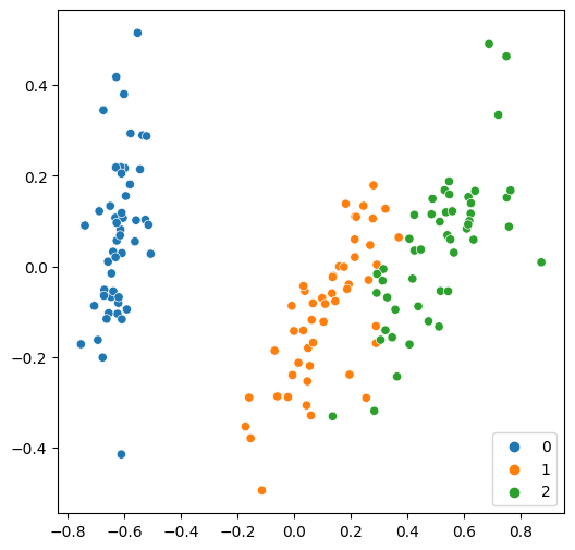
We transform our four features into two features only. This dimensionality reduction is for educational purposes only. As you saw in the previous section, we can train a quantum model using all four features from the dataset.

Now, we can easily plot these two features on a single figure.

from sklearn.decomposition import PCA

features = PCA(n_components=2).fit_transform(features)

plt.rcParams["figure.figsize"] = (6, 6)
sns.scatterplot(x=features[:, 0], y=features[:, 1], hue=labels, palette="tab10")

<AxesSubplot:>

As usual, we split the dataset first, then fit a classical model.

train_features, test_features, train_labels, test_labels = train_test_split(
    features, labels, train_size=0.8, random_state=algorithm_globals.random_seed
)

svc.fit(train_features, train_labels)

train_score_c2 = svc.score(train_features, train_labels)
test_score_c2 = svc.score(test_features, test_labels)

print(f"Classical SVC on the training dataset: {train_score_c2:.2f}")
print(f"Classical SVC on the test dataset:     {test_score_c2:.2f}")

Classical SVC on the training dataset: 0.97
Classical SVC on the test dataset:     0.90

The results are still good but slightly worse compared to the initial version. Let’s see how a quantum model deals with them. As we now have two qubits, we must recreate the feature map and ansatz.

num_features = features.shape[1]

feature_map = ZZFeatureMap(feature_dimension=num_features, reps=1)
ansatz = RealAmplitudes(num_qubits=num_features, reps=3)

We also reduce the maximum number of iterations we run the optimization process for, as we expect it to converge faster because we now have fewer qubits.

optimizer = COBYLA(maxiter=40)

Now we construct a quantum classifier from the new parameters and train it.

vqc = VQC(
    sampler=sampler,
    feature_map=feature_map,
    ansatz=ansatz,
    optimizer=optimizer,
    callback=callback_graph,
)

# clear objective value history
objective_func_vals = []

# make the objective function plot look nicer.
plt.rcParams["figure.figsize"] = (12, 6)


start = time.time()
vqc.fit(train_features, train_labels)
elapsed = time.time() - start

print(f"Training time: {round(elapsed)} seconds")

Training time: 58 seconds

train_score_q2_ra = vqc.score(train_features, train_labels)
test_score_q2_ra = vqc.score(test_features, test_labels)

print(f"Quantum VQC on the training dataset using RealAmplitudes: {train_score_q2_ra:.2f}")
print(f"Quantum VQC on the test dataset using RealAmplitudes:     {test_score_q2_ra:.2f}")

Quantum VQC on the training dataset using RealAmplitudes: 0.58
Quantum VQC on the test dataset using RealAmplitudes:     0.63

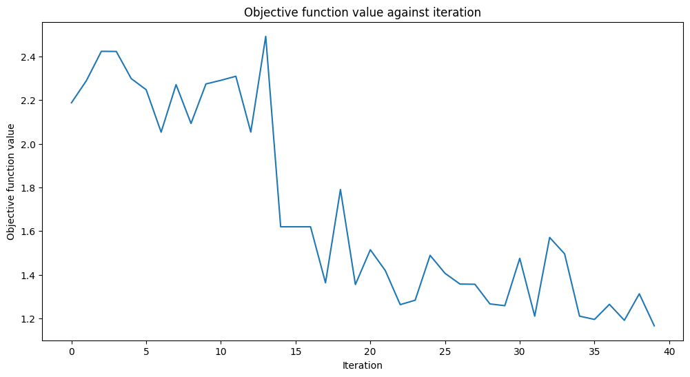
Well, the scores are higher than a fair coin toss but could be better. The objective function is almost flat towards the end, meaning increasing the number of iterations won’t help, and model performance will stay the same. Let’s see what we can do with another ansatz.

from qiskit.circuit.library import EfficientSU2

ansatz = EfficientSU2(num_qubits=num_features, reps=3)
optimizer = COBYLA(maxiter=40)

vqc = VQC(
    sampler=sampler,
    feature_map=feature_map,
    ansatz=ansatz,
    optimizer=optimizer,
    callback=callback_graph,
)

# clear objective value history
objective_func_vals = []

start = time.time()
vqc.fit(train_features, train_labels)
elapsed = time.time() - start

print(f"Training time: {round(elapsed)} seconds")

Training time: 74 seconds

train_score_q2_eff = vqc.score(train_features, train_labels)
test_score_q2_eff = vqc.score(test_features, test_labels)

print(f"Quantum VQC on the training dataset using EfficientSU2: {train_score_q2_eff:.2f}")
print(f"Quantum VQC on the test dataset using EfficientSU2:     {test_score_q2_eff:.2f}")

Quantum VQC on the training dataset using EfficientSU2: 0.78
Quantum VQC on the test dataset using EfficientSU2:     0.80

The scores are better than in the previous setup. Perhaps if we had used more iterations, we could do even better.

5. Conclusion

In this tutorial, we have built two classical and three quantum machine learning models. Let’s print an overall table with our results.

print(f"Model                           | Test Score | Train Score")
print(f"SVC, 4 features                 | {train_score_c4:10.2f} | {test_score_c4:10.2f}")
print(f"VQC, 4 features, RealAmplitudes | {train_score_q4:10.2f} | {test_score_q4:10.2f}")
print(f"----------------------------------------------------------")
print(f"SVC, 2 features                 | {train_score_c2:10.2f} | {test_score_c2:10.2f}")
print(f"VQC, 2 features, RealAmplitudes | {train_score_q2_ra:10.2f} | {test_score_q2_ra:10.2f}")
print(f"VQC, 2 features, EfficientSU2   | {train_score_q2_eff:10.2f} | {test_score_q2_eff:10.2f}")

Model                           | Test Score | Train Score
SVC, 4 features                 |       0.99 |       0.97
VQC, 4 features, RealAmplitudes |       0.85 |       0.87
----------------------------------------------------------
SVC, 2 features                 |       0.97 |       0.90
VQC, 2 features, RealAmplitudes |       0.58 |       0.63
VQC, 2 features, EfficientSU2   |       0.78 |       0.80

Unsurprisingly, the classical models perform better than their quantum counterparts, but classical ML has come a long way, and quantum ML has yet to reach that level of maturity. As we can see, we achieved the best results using a classical support vector machine. But the quantum model trained on four features was also quite good. When we reduced the number of features, the performance of all models went down as expected. So, if resources permit training a model on a full-featured dataset without any reduction, you should train such a model. If not, you may expect to compromise between dataset size, training time, and score.

Another observation is that even a simple ansatz change can lead to better results. The two-feature model with the EfficientSU2 ansatz performs better than the one with RealAmplitudes. That means the choice of hyperparameters plays the same critical role in quantum ML as in classical ML, and searching for optimal hyperparameters may take a long time. You may apply the same techniques we use in classical ML, such as random/grid or more sophisticated approaches.

We hope this brief tutorial helps you to take the leap from classical to quantum ML.

import qiskit.tools.jupyter

%qiskit_version_table
%qiskit_copyright

Version Information

Qiskit Software	Version
qiskit-terra	0.22.0
qiskit-aer	0.11.0
qiskit-ignis	0.7.0
qiskit	0.33.0
qiskit-machine-learning	0.5.0
System information
Python version	3.7.9
Python compiler	MSC v.1916 64 bit (AMD64)
Python build	default, Aug 31 2020 17:10:11
OS	Windows
CPUs	4
Memory (Gb)	31.837730407714844
Fri Oct 14 14:33:06 2022 GMT Daylight Time

This code is a part of Qiskit

© Copyright IBM 2017, 2022.

This code is licensed under the Apache License, Version 2.0. You may
obtain a copy of this license in the LICENSE.txt file in the root directory
of this source tree or at http://www.apache.org/licenses/LICENSE-2.0.

Any modifications or derivative works of this code must retain this
copyright notice, and modified files need to carry a notice indicating
that they have been altered from the originals.