Note
இந்தப் பக்கம் docs/tutorials/12_quantum_autoencoder.ipynb இலிருந்து உருவாக்கப்பட்டது.
குவாண்டம் ஆட்டோஎன்கோடர்#
இந்த டுடோரியலின் குறிக்கோள், குவாண்டம் ஆட்டோஎன்கோடரை உருவாக்குவதாகும், இது ஒரு குவாண்டம் நிலையைச் சிறிய அளவிலான குவிட்களில் சுருக்கக்கூடிய ஒரு சுற்று, அதே நேரத்தில் ஆரம்ப நிலையிலிருந்து தகவலைத் தக்கவைத்துக்கொள்ளும்.
இந்த டுடோரியல் முழுவதும், ஒரு குவாண்டம் ஆட்டோஎன்கோடரின் கட்டமைப்பையும், தகவலை சுருக்கி குறியாக்குவதற்கும் அத்தகைய அமைப்பை எவ்வாறு வடிவமைத்து பயிற்சியளிக்கலாம் என்பதை விளக்குகிறோம். இந்த விவாதத்தைத் தொடர்ந்து, வெவ்வேறு குவாண்டம் நிலைகளை சுருக்கவும், பூஜ்ஜியங்கள் மற்றும் ஒன்றின் படங்களை சுருக்கும் திறனையும் அத்தகைய அமைப்பின் திறன்களை நிரூபிக்க இரண்டு எடுத்துக்காட்டுகளைத் தருகிறோம்.
உள்ளடக்கம்#
பின்வரும் பயிற்சி பின்வருமாறு பிரிக்கப்பட்டுள்ளது:
ஆட்டோஎன்கோடர் என்றால் என்ன?
குவாண்டம் ஆட்டோஎன்கோடர்
குவாண்டம் ஆட்டோஎன்கோடரின் கூறுகள்
இழப்பு செயல்பாட்டைத் தேர்ந்தெடுப்பது
எங்கள் ஆட்டோஎன்கோடரை உருவாக்குகிறது
ஒரு எளிய உதாரணம்: டொமைன் வால்
இலக்கங்களின் சத்தமில்லாத படங்களுக்கான குவாண்டம் ஆட்டோஎன்கோடர்
குவாண்டம் ஆட்டோஎன்கோடரின் பயன்பாடுகள்
குறிப்புகள்
1. ஆட்டோஎன்கோடர் என்றால் என்ன?#
கிளாசிக்கல் ஆட்டோஎன்கோடர் (CAE) என்பது ஒரு வகையான நரம்பியல் நெட்வொர்க் கட்டமைப்பாகும், இது பொதுவாகப் பிரதிநிதித்துவக் கற்றலைப் பயன்படுத்தி உள்ளீட்டிலிருந்து தகவலைத் திறம்பட சுருக்கவும் குறியாக்கவும் பயன்படுகிறது. சுருக்கத்தைத் தொடர்ந்து, டிகோடரைப் பயன்படுத்தி ஒருவர் தரவைச் சுருக்கலாம்.
படம் 1 இல் காணப்படுவது போல், வழக்கமான தன்னியக்க குறியாக்கிகள் பொதுவாக மூன்று அடுக்குகளாகப் பிரிக்கப்படுகின்றன.
 படம் 1: உள்ளீடு, இடையூறு மற்றும் வெளியீட்டு அடுக்கு ஆகியவற்றை உள்ளடக்கிய கிளாசிக்கல் ஆட்டோஎன்கோடரின் எடுத்துக்காட்டு.
முதல் அடுக்கு உள்ளீட்டு அடுக்கு (1) என்று அழைக்கப்படுகிறது, மேலும் இது நமது நீளம் \(n\) தரவை உள்ளிடும் அடுக்கு ஆகும்.
உள்ளீட்டுத் தரவு பின்னர் ஒரு குறியாக்கி வழியாகச் சென்று அடுத்த லேயருக்குப் பயணிக்கிறது, இது குறைவான முனைகளைக் கொண்டது அல்லது பரிமாணங்களில் குறைக்கப்பட்டு பாட்டில்நெக் லேயர் (2) என அழைக்கப்படுகிறது. உள்ளீடு அடுக்கு இந்தச் செயல்முறைமூலம் சுருக்கப்பட்டது. பொதுவான CAEகள் பல அடுக்குகளைக் கொண்டிருக்கலாம்.
இறுதி அடுக்கு அவுட்புட் லேயர் (3) என்று அழைக்கப்படுகிறது. இங்கே சுருக்கப்பட்ட தரவு அதன் அசல் அளவு, \(n\), சுருக்கப்பட்ட தரவிலிருந்து ஒரு குறிவிலக்கியின் செயல்முறைமூலம் மறுகட்டமைக்கப்படுகிறது.
எங்கள் உள்ளீட்டுத் தரவை CAE மூலம் அனுப்புவதன் மூலம், உள்ளீட்டுத் தரவிலிருந்து முடிந்தவரை தகவல்களைத் தக்கவைத்துக்கொள்ளும் அதே வேளையில், இடையூறு அடுக்கில் காணப்படுவது போல், நமது உள்ளீட்டுத் தரவின் பரிமாணத்தைக் குறைக்க முடியும். இந்த அம்சத்தின் காரணமாக, CAE இன் பொதுவான பயன்பாடுகள் இமேஜ் டெனாயிசிங், அனோமாலி கண்டறிதல் மற்றும் முக அங்கீகார சாதனங்கள் ஆகும். கிளாசிக்கல் ஆட்டோஎன்கோடர்கள் பற்றிய கூடுதல் தகவலுக்கு, [1] பார்க்கவும்.
2. குவாண்டம் ஆட்டோஎன்கோடர்#
குவாண்டம் ஆட்டோஎன்கோடரான CAEக்கு ஒரு குவாண்டம் எண்ணையும் நாம் வரையறுக்கலாம். CAE ஐப் போலவே, குவாண்டம் ஆட்டோஎன்கோடரும் நரம்பியல் நெட்வொர்க்கின் உள்ளீட்டின் பரிமாணத்தைக் குறைப்பதை நோக்கமாகக் கொண்டுள்ளது, இந்த விஷயத்தில் ஒரு குவாண்டம் நிலை. இதன் சித்திரப் பிரதிபலிப்பை படம் 2 இல் காணலாம்.
 படம் 2: குவாண்டம் ஆட்டோஎன்கோடரின் சித்திரப் பிரதிநிதித்துவம். CAE உடனான ஒற்றுமையை இங்கே காணலாம், சுற்று ஒரு உள்ளீட்டு நிலை, இடையூறு நிலை மற்றும் வெளியீட்டு நிலை ஆகியவற்றைக் கொண்டுள்ளது.
அதன் கிளாசிக்கல் எண்ணைப் போலவே, எங்கள் சுற்று மூன்று அடுக்குகளைக் கொண்டுள்ளது. முதலில் நமது நிலையை உள்ளிடுகிறோம் \(|\psi>\) (இதில் \(n\) qubits உள்ளது), அதில் நாம் சுருக்க விரும்புகிறோம். இது எங்கள் உள்ளீட்டு அடுக்கு (1).
We then apply our parametrized circuit on our input state, which will act as our encoder and 'compresses' our quantum state, reducing the dimensionality of our state to \(n-k\) qubits. Our new compressed state is of the form \(|\psi_{comp}> \otimes |0>^{\otimes k}\), where \(|\psi_{comp}>\) contains \(n-k\) qubits.
இந்த அளவுருப்படுத்தப்பட்ட சுற்று அளவுருக்களின் தொகுப்பைப் பொறுத்தது, இது எங்கள் குவாண்டம் ஆட்டோஎன்கோடரின் முனைகளாக இருக்கும். பயிற்சி செயல்முறை முழுவதும், இழப்புச் செயல்பாட்டை மேம்படுத்த இந்த அளவுருக்கள் புதுப்பிக்கப்படும்.
மீதமுள்ள சர்க்யூட்டின் மீதமுள்ள \(k\) குவிட்களை நாங்கள் புறக்கணிக்கிறோம். இது எங்களின் பிளாட்நெக் லேயர் (2) மற்றும் எங்கள் உள்ளீட்டு நிலை இப்போது சுருக்கப்பட்டுள்ளது.
The final layer consists of the addition of \(k\) qubits (all in the state \(|0\rangle\)) and applying another parametrized circuit between the compressed state and the new qubits. This parametrized circuit acts as our decoder and reconstructs the input state from the compressed state using the new qubits. After the decoder, we retain the original state as the state travels to the output layer (3).
3. Components of a Quantum Autoencoder#
Before building our Quantum Autoencoder, we must note a few subtleties.
We first note that we cannot introduce or disregard qubits in the middle of a Quantum Circuit when implementing an autoencoder using Qiskit.
Because of this we must include our reference state as well as our auxiliary qubits (whose role will be described in later sections) at the beginning of the circuit.
Therefore our input state will consist of our input state, reference state and one auxiliary qubit, as well as a classical register to perform measurements (which will be described in the next section). A pictorial representation of this can be seen in Figure 3.
 Figure 3: Pictorial Representation of input state of Quantum Autoencoder. Note that we must also include an auxiliary qubit, the reference state and classical register at the beginning of the circuit, even though they are not used until later in the circuit.
4. Choosing a Loss Function#
We now define our cost function, which we will use to train our Quantum Autoencoder, to return the input state. There’s a bit of math involved here, so skip this section if you’re not interested!
We take the cost function as defined in [2], which tries to maximize the fidelity between the input and output state of our Quantum Autoencoder.
We first define subsystems \(A\) and \(B\) to contain \(n\) and \(k\) qubits respectively, while \(B'\) is the space which will contain our reference space. We call the subsystem \(A\) our latent space, which will contain the compressed qubit state, and \(B\) our trash space, which contain the qubits of which we disregard throughout compression.
Our input state therefore \(|\psi_{AB}>\) contains \(n + k\) qubits. We define the reference space \(B'\) which contains the reference state \(|a>_{B'}\). This space will contain the additional \(k\) qubits we use in the decoder. All of these subsystems can be seen in Figure 3.
We define the parameterized circuit as \(U(\theta)\) which we will use as our encoder. However the structure and parameters of our parametrized circuit is currently unknown to us and may vary for different input states. To determine the parameters to compress our input state, we must train our device to maximally compress the state by adjusting the values of the parameters \(\theta\). For the decoder we will use \(U^{\dagger}(\theta)\).
Our goal therefore is to maximize the fidelity between the input and output states, i.e.
where
We can maximize this fidelity by tuning the parameters \(\theta\) in our parametrized circuit. However, this fidelity can at times be complicated to determine and may require a large amount of gates needed to calculate the fidelity between two states, i.e. the larger the number of qubits, the more gates required which results to deeper circuits. Therefore we look for alternative means of comparing the input and output states.
As shown in [2] a simpler way of determining an optimally compressed state is to perform a swap gate between the trash state and reference state. These states usually have a smaller number of qubits and are therefore easier to compare, due to the smaller amount of gates required. As shown in [2] maximizing the fidelity of such these two states is equivalent to maximizing the fidelity of the input and output state and thus determining an optimal compression of our input circuit.
Keeping our reference state fixed, our cost function will now be a function of the trash state and is denoted as;
Throughout the training process, we adjust the parameters \(\theta\) in our encoder and perform a swap test (as described below) to determine the fidelity between these trash and reference states. In doing so, we must include an additional qubit, our auxiliary qubit, which will be used throughout the swap test and measured to determine the overall fidelity of the trash and reference states. This is the reason why we included both an auxiliary qubit and classical register in the previous section when initializing our circuit.
The SWAP Test#
The SWAP Test is a procedure commonly used to compare two states by applying CNOT gates to each qubit (for further information see [3]). By running the circuit \(M\) times, and applying the SWAP test, we then measure the auxiliary qubit. We use the number of states in the state \(|1\rangle\) to compute:
where \(L\) is the count for the states in the \(|1\rangle\) state. As shown in [3], maximizing this function corresponds to the two states of which we are comparing being identical. We therefore aim to maximize this function, i.e. minimize \(\frac{2}{M}L\). This value will be therefore be our cost function.
5. Building the Quantum Autoencoder Ansatz#
First, we implement IBM’s Qiskit to build our Quantum Autoencoder. We first begin by importing in the necessary libraries and fixing the seed.
[1]:
import json
import time
import warnings

import matplotlib.pyplot as plt
import numpy as np
from IPython.display import clear_output
from qiskit import ClassicalRegister, QuantumRegister
from qiskit import QuantumCircuit
from qiskit.circuit.library import RealAmplitudes
from qiskit.quantum_info import Statevector
from qiskit_algorithms.optimizers import COBYLA
from qiskit_algorithms.utils import algorithm_globals

from qiskit_machine_learning.circuit.library import RawFeatureVector
from qiskit_machine_learning.neural_networks import SamplerQNN

algorithm_globals.random_seed = 42
We begin by defining our parametrized ansatz for the Quantum Autoencoder. This will be our parametrized circuit where we can tune the parameters to maximize the fidelity between the trash and reference states.
The Parametrized Circuit#
The parametrized circuit we will use below for our encoder is the RealAmplitude Ansatz available in Qiskit. One of the reasons why we have chosen this ansatz is because it is a 2-local circuit, the prepared quantum states will only have real amplitudes, and does not rely on full connectivity between each qubits, which is hard to implement or can lead to deep circuits.
We define our parametrized circuit for our Encoder below, where we set the repetition parameter to reps=5, to increase the number of parameters in our circuit allowing greater flexibility.
[2]:
def ansatz(num_qubits):
    return RealAmplitudes(num_qubits, reps=5)
Let’s draw this ansatz with \(5\) qubits and see what it looks like.
[3]:
num_qubits = 5
circ = ansatz(num_qubits)
circ.decompose().draw("mpl")
[3]:

We now apply this Encoder to the state we wish to compress. In this example, we divide our initial \(5\) qubit state into a \(3\) qubit latent state (\(n = 3\)) and \(2\) qubit trash space (\(k = 2\)).
முந்தைய பகுதியில் விளக்கியது போல், நமது சர்க்யூட்டில் ஒரு \(2\) குவிட் ரெஃபரன்ஸ் ஸ்பேஸையும், குறிப்பு மற்றும் குப்பை நிலைகளுக்கு இடையே ஸ்வாப் சோதனையைச் செய்ய ஒரு துணை குவிட்டையும் சேர்க்க வேண்டும். எனவே எங்கள் சர்க்யூட்டில் மொத்தம் \(2 + 3 + 2 + 1 = 8\) qubits மற்றும் \(1\) கிளாசிக்கல் பதிவேடு இருக்கும்.
எங்கள் நிலையைத் துவக்கிய பிறகு, நாங்கள் எங்கள் அளவுரு சுற்றுகளைப் பயன்படுத்துகிறோம்.
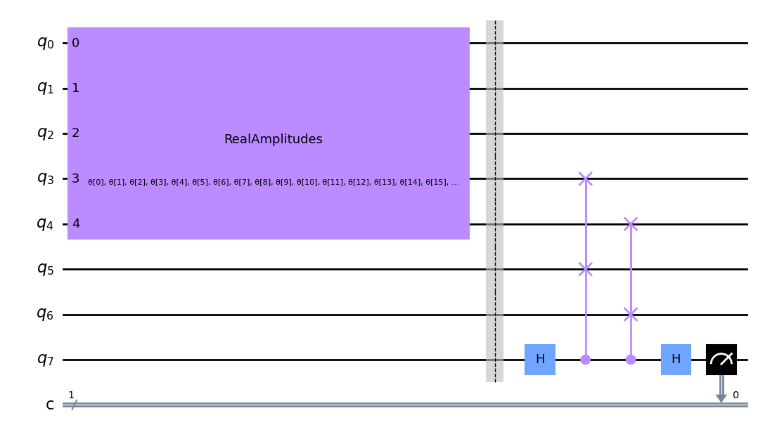
இதைத் தொடர்ந்து, நமது ஆரம்ப நிலையை மறைந்த இடம் (அழுத்தப்பட்ட நிலை) மற்றும் குப்பை இடம் (நாம் புறக்கணிக்கும் மாநிலத்தின் பகுதி) எனப் பிரித்து, குறிப்பு நிலைக்கும் குப்பை இடத்துக்கும் இடையில் இடமாற்றுச் சோதனையைச் செய்கிறோம். குறிப்பு மற்றும் குப்பை நிலைகளுக்கு இடையிலான நம்பகத்தன்மையை தீர்மானிக்க கடைசி குவிட் அளவிடப்படுகிறது. இதன் ஒரு சித்திரப் பிரதிநிதித்துவம் படம் 4 இல் கீழே கொடுக்கப்பட்டுள்ளது.

படம் 4: பயிற்சி செயல்பாட்டில் குவாண்டம் ஆட்டோஎன்கோடரின் எடுத்துக்காட்டு. குப்பைக்கும் குறிப்பு இடத்துக்கும் இடையே உள்ள நம்பகத்தன்மையைத் தீர்மானிக்க, இடமாற்று சோதனையைப் பயன்படுத்துகிறோம்.
மேலே உள்ள சர்க்யூட் உள்ளமைவை \(5\) qubit டொமைன் சுவர் நிலை \(|00111\rangle\) க்கு செயல்படுத்த கீழே ஒரு செயல்பாட்டை வரையறுத்து, கீழே ஒரு உதாரணத்தைத் திட்டமிடுகிறோம். இங்கே qubits \(5\) மற்றும் \(6\) என்பது குறிப்பு நிலை, \(0, 1, 2, 3, 4\) ஆகியவை நாம் சுருக்கி குவிட் செய்ய விரும்பும் ஆரம்ப நிலை \(7\) ஸ்வாப் சோதனையில் பயன்படுத்தப்படும் எங்கள் துணை குவிட் ஆகும். இடமாற்று சோதனையில் qubit \(7\) இன் முடிவுகளை அளவிடுவதற்கு ஒரு கிளாசிக்கல் பதிவேட்டையும் சேர்த்துள்ளோம்.
[4]:
def auto_encoder_circuit(num_latent, num_trash):
    qr = QuantumRegister(num_latent + 2 * num_trash + 1, "q")
    cr = ClassicalRegister(1, "c")
    circuit = QuantumCircuit(qr, cr)
    circuit.compose(ansatz(num_latent + num_trash), range(0, num_latent + num_trash), inplace=True)
    circuit.barrier()
    auxiliary_qubit = num_latent + 2 * num_trash
    # swap test
    circuit.h(auxiliary_qubit)
    for i in range(num_trash):
        circuit.cswap(auxiliary_qubit, num_latent + i, num_latent + num_trash + i)

    circuit.h(auxiliary_qubit)
    circuit.measure(auxiliary_qubit, cr[0])
    return circuit


num_latent = 3
num_trash = 2
circuit = auto_encoder_circuit(num_latent, num_trash)
circuit.draw("mpl")
[4]:
அசல் உள்ளீட்டு நிலையை மறுகட்டமைப்பதற்காக, ஸ்வாப் சோதனைக்குப் பிறகு, நமது அளவுரு சுற்றுவட்டத்தின் இணைப்பினைப் பயன்படுத்த வேண்டும். இருப்பினும், பயிற்சியின் போது, குப்பை நிலை மற்றும் குறிப்பு நிலை ஆகியவற்றில் மட்டுமே நாங்கள் ஆர்வமாக உள்ளோம். எனவே, எங்கள் ஆரம்ப உள்ளீட்டை மறுகட்டமைக்க விரும்பும் வரை சுருக்கத்தைத் தொடர்ந்து வாயில்களை விலக்கலாம்.
எங்கள் குவாண்டம் ஆட்டோஎன்கோடரை உருவாக்கியபிறகு, அடுத்த கட்டமாக, எங்கள் குவாண்டம் ஆட்டோஎன்கோடரைப் பயிற்றுவித்து, நிலையைச் சுருக்கவும், செலவுச் செயல்பாட்டை அதிகரிக்கவும் மற்றும் அளவுருக்கள் \(\theta\) தீர்மானிக்கவும்.
6. ஒரு எளிய உதாரணம்: டொமைன் வால் ஆட்டோஎன்கோடர்#
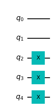
Let’s first begin with a simple example, a state known as the Domain Wall, which for \(5\) qubits is given by \(|00111\rangle\). Here we will try and compress this state from \(5\) qubits to \(3\) qubits, with the remaining qubits in the trash space, in the state \(|00\rangle\). We can create a function to build the domain wall state below.
[5]:
def domain_wall(circuit, a, b):
    # Here we place the Domain Wall to qubits a - b in our circuit
    for i in np.arange(int(b / 2), int(b)):
        circuit.x(i)
    return circuit


domain_wall_circuit = domain_wall(QuantumCircuit(5), 0, 5)
domain_wall_circuit.draw("mpl")
[5]:
Now let’s train our Autoencoder to compress this state from 5 qubits to 3 qubits (qubits 0,1 and 2), with the remaining qubits in the trash space (qubits 3 and 4) being in the |00> state.
பிரிவு 4 இல் விவரிக்கப்பட்டுள்ளபடி, இழப்புச் செயல்பாட்டில் பயன்படுத்துவதற்கு ஒரு சர்க்யூட்டை உருவாக்குகிறோம், இது எங்கள் குறிப்பிட்ட ஆட்டோஎன்கோடர் செயல்பாட்டிற்கான ஸ்வாப் சோதனையைப் பயன்படுத்தி கீழே உள்ள இரண்டு நிலைகளுக்கு இடையே உள்ள நம்பகத்தன்மையை தீர்மானிக்கிறது. ஸ்வாப் சோதனை பற்றிய கூடுதல் தகவலுக்கு, [1] பார்க்கவும்.
[6]:
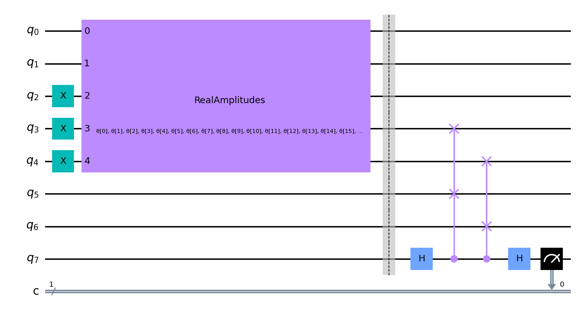
ae = auto_encoder_circuit(num_latent, num_trash)
qc = QuantumCircuit(num_latent + 2 * num_trash + 1, 1)
qc = qc.compose(domain_wall_circuit, range(num_latent + num_trash))
qc = qc.compose(ae)
qc.draw("mpl")
[6]:
பின்னர், நாம் ஒரு குவாண்டம் நரம்பியல் வலையமைப்பை உருவாக்கி, சுற்றுகளை ஒரு அளவுருவாக அனுப்புகிறோம். இந்த நெட்வொர்க் ஒரு விளக்கம் செயல்பாட்டை எடுக்க வேண்டும் என்பதை நாங்கள் கவனிக்கிறோம், இது நெட்வொர்க்கின் வெளியீட்டை வெளியீட்டு வடிவத்திற்கு எவ்வாறு வரைபடமாக்குகிறது என்பதை தீர்மானிக்கிறது. நாம் ஒரே ஒரு குவிட்டை மட்டும் அளப்பதால், நெட்வொர்க்கின் வெளியீடு \(0\) அல்லது \(1\), எனவே வெளியீடு வடிவம் \(2\), சாத்தியமான விளைவுகளின் எண்ணிக்கை. பின்னர், நாங்கள் ஒரு அடையாள வரைபடத்தை அறிமுகப்படுத்துகிறோம். நெட்வொர்க்கின் வெளியீடு என்பது விளக்கம்-மேப் செய்யப்பட்ட பிட் சரங்களைப் பெறுவதற்கான நிகழ்தகவுகளின் திசையன் ஆகும். எனவே, நாம் \(0\) அல்லது \(1\) பெறுவதற்கான நிகழ்தகவுகளைப் பெறுகிறோம், இதைத்தான் நாம் தேடுகிறோம். செலவுச் செயல்பாட்டில் நாம் \(1\) பெறுவதற்கான நிகழ்தகவைப் பயன்படுத்துகிறோம் மற்றும் \(1\) க்கு வழிவகுக்கும் விளைவுகளை அபராதம் விதிக்கிறோம், எனவே குப்பை இடம் மற்றும் குறிப்பு இடைவெளி இடையே நம்பகத்தன்மையை அதிகரிக்கிறது.
[7]:
# Here we define our interpret for our SamplerQNN
def identity_interpret(x):
    return x


qnn = SamplerQNN(
    circuit=qc,
    input_params=[],
    weight_params=ae.parameters,
    interpret=identity_interpret,
    output_shape=2,
)
அடுத்து, எங்கள் செலவு செயல்பாட்டை உருவாக்குகிறோம். முந்தைய பிரிவில் விவரிக்கப்பட்டுள்ளபடி, எங்கள் நோக்கம் \(\frac{2}{M}L\) ஐக் குறைப்பதாகும், இது \(|1\rangle\) நிலையில் இறுதி குவிட்டைப் பெறுவதற்கான இரு மடங்கு நிகழ்தகவு ஆகும். . எனவே குவிட் 7 இல் \(|1\rangle\) பெறுவதைக் குறைக்க விரும்புகிறோம்.
ஒவ்வொரு செலவுச் செயல்பாட்டின் மதிப்பீட்டிலும் செலவுச் செயல்பாடு புறநிலை மதிப்பைக் குறிக்கும்.
[8]:
def cost_func_domain(params_values):
    probabilities = qnn.forward([], params_values)
    # we pick a probability of getting 1 as the output of the network
    cost = np.sum(probabilities[:, 1])

    # plotting part
    clear_output(wait=True)
    objective_func_vals.append(cost)
    plt.title("Objective function value against iteration")
    plt.xlabel("Iteration")
    plt.ylabel("Objective function value")
    plt.plot(range(len(objective_func_vals)), objective_func_vals)
    plt.show()
    return cost
இப்போது ஹில்பர்ட் இடத்தின் பரிமாணத்தை \(5\) qubits இலிருந்து \(3\) ஆகக் குறைக்க எங்கள் ஆட்டோஎன்கோடரைப் பயிற்றுவிப்போம் ,மாநிலத்தில் குப்பை இடத்தை விட்டு வெளியேறும்போது \(|00\rangle\).நாம் ஆரம்பத்தில் அளவுருக்களை \(\theta\) ஐ சீரற்ற மதிப்புகளாக அமைத்து, COBYLA ஆப்டிமைசரைப் பயன்படுத்துவதன் மூலம் எங்கள் செலவுச் செயல்பாட்டைக் குறைக்க இந்த அளவுருக்களை டியூன் செய்கிறோம்.
[9]:
opt = COBYLA(maxiter=150)
initial_point = algorithm_globals.random.random(ae.num_parameters)

objective_func_vals = []
# make the plot nicer
plt.rcParams["figure.figsize"] = (12, 6)

start = time.time()
opt_result = opt.minimize(cost_func_domain, initial_point)
elapsed = time.time() - start

print(f"Fit in {elapsed:0.2f} seconds")
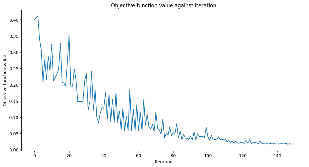
Fit in 18.48 seconds
Looks like it has converged! After training our Quantum Autoencoder, let’s build it and see how well it compresses the state!
இதைச் செய்ய, முதலில் எங்கள் ஆட்டோஎன்கோடரை ஒரு \(5\) qubit டொமைன் வால் நிலைக்குப் பயன்படுத்துகிறோம். இந்த நிலையைப் பயன்படுத்திய பிறகு, சுருக்கப்பட்ட நிலை \(|00\rangle\) வடிவத்தில் இருக்க வேண்டும். எனவே கடைசி இரண்டு குவிட்களை மீட்டமைப்பது நமது எல்லா நிலையிலும் பாதிப்பை ஏற்படுத்தாது.
மீட்டமைத்த பிறகு, நாங்கள் எங்கள் டிகோடரைப் பயன்படுத்துகிறோம் (எங்கள் குறியாக்கியின் ஹெர்மிஷியன் கான்ஜுகேட்) மற்றும் நம்பகத்தன்மையைத் தீர்மானிப்பதன் மூலம் அதை ஆரம்ப நிலைக்கு ஒப்பிடுவோம். எங்கள் நம்பகத்தன்மை ஒன்று எனில், எங்கள் ஆட்டோஎன்கோடர், டொமைன் சுவரின் அனைத்துத் தகவலையும் திறமையாக ஒரு சிறிய குவிட்களில் குறியாக்கம் செய்து, டிகோடிங் செய்யும் போது, அசல் நிலையைத் தக்கவைத்துக் கொள்கிறோம்!
Let’s first apply our circuit to the Domain Wall State, using the parameters we obtained when training our Quantum Autoencoder. (Note we have included barriers in our circuit below, however these are not necessary for the implementation of the Quantum Autoencoder and are used to determine between different sections of our circuit).
[10]:
test_qc = QuantumCircuit(num_latent + num_trash)
test_qc = test_qc.compose(domain_wall_circuit)
ansatz_qc = ansatz(num_latent + num_trash)
test_qc = test_qc.compose(ansatz_qc)
test_qc.barrier()
test_qc.reset(4)
test_qc.reset(3)
test_qc.barrier()
test_qc = test_qc.compose(ansatz_qc.inverse())

test_qc.draw("mpl")
[10]:

இப்போது பயிற்சியில் பெறப்பட்ட அளவுரு மதிப்புகளை நாங்கள் ஒதுக்குகிறோம்.
[11]:
test_qc = test_qc.assign_parameters(opt_result.x)
Now let’s get the statevectors of our Domain Wall state and output circuit and calculate the fidelity!
[12]:
domain_wall_state = Statevector(domain_wall_circuit).data
output_state = Statevector(test_qc).data

fidelity = np.sqrt(np.dot(domain_wall_state.conj(), output_state) ** 2)
print("Fidelity of our Output State with our Input State: ", fidelity.real)
Fidelity of our Output State with our Input State: 0.9832814006314854
எங்கள் நம்பகத்தன்மை மிகவும் அதிகமாக இருப்பதை நீங்கள் பார்க்க முடியும், மேலும் எங்கள் ஆட்டோஎன்கோடர் எங்கள் தரவுத்தொகுப்பைச் சுருக்கி உள்ளீடு நிலையிலிருந்து அனைத்து தகவல்களையும் தக்க வைத்துக் கொண்டது!
பூஜ்ஜியம் மற்றும் ஒன்று எண்களின் படங்கள் போன்ற சத்தம் கொண்ட மிகவும் சிக்கலான தரவுத்தொகுப்புகளுக்கு அத்தகைய குவாண்டம் ஆட்டோஎன்கோடரைப் பயன்படுத்த முடியுமா என்று இப்போது பார்ப்போம்.
7. டிஜிட்டல் சுருக்கத்திற்கான குவாண்டம் ஆட்டோஎன்கோடர்#
தரவுத்தொகுப்பை சுருக்க கையால் எழுதப்பட்ட இலக்கங்களின் தொகுப்பு போன்ற மிகவும் சிக்கலான எடுத்துக்காட்டுகளுக்கு குவாண்டம் ஆட்டோஎன்கோடரைப் பயன்படுத்தலாம். குவாண்டம் கம்ப்யூட்டரில் தரவை மிகவும் திறமையாகச் சேமிக்கும் திறனைக் கொடுத்து, அத்தகைய உதாரணத்தை சுருக்க, குவாண்டம் ஆட்டோஎன்கோடரைப் பயிற்றுவிக்க முடியும் என்பதை கீழே காண்பிப்போம்.
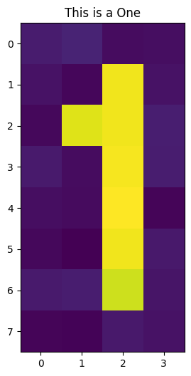
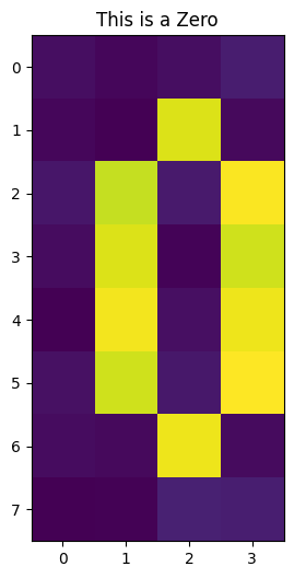
இந்த டுடோரியலுக்காக, பூஜ்ஜியங்கள் மற்றும் ஒன்றைக் கொண்ட சத்தமில்லாத தரவுத்தொகுப்பிற்காகக் குவாண்டம் ஆட்டோஎன்கோடரை உருவாக்குவோம், அதைக் கீழே காணலாம்.
Each image contains \(32\) pixels of which can be encoded into \(5\) qubits by Amplitude Encoding. This can be done using Qiskit Machine Learning’s RawFeatureVector feature map.
[13]:
def zero_idx(j, i):
    # Index for zero pixels
    return [
        [i, j],
        [i - 1, j - 1],
        [i - 1, j + 1],
        [i - 2, j - 1],
        [i - 2, j + 1],
        [i - 3, j - 1],
        [i - 3, j + 1],
        [i - 4, j - 1],
        [i - 4, j + 1],
        [i - 5, j],
    ]


def one_idx(i, j):
    # Index for one pixels
    return [[i, j - 1], [i, j - 2], [i, j - 3], [i, j - 4], [i, j - 5], [i - 1, j - 4], [i, j]]


def get_dataset_digits(num, draw=True):
    # Create Dataset containing zero and one
    train_images = []
    train_labels = []
    for i in range(int(num / 2)):
        # First we introduce background noise
        empty = np.array([algorithm_globals.random.uniform(0, 0.1) for i in range(32)]).reshape(
            8, 4
        )

        # Now we insert the pixels for the one
        for i, j in one_idx(2, 6):
            empty[j][i] = algorithm_globals.random.uniform(0.9, 1)
        train_images.append(empty)
        train_labels.append(1)
        if draw:
            plt.title("This is a One")
            plt.imshow(train_images[-1])
            plt.show()

    for i in range(int(num / 2)):
        empty = np.array([algorithm_globals.random.uniform(0, 0.1) for i in range(32)]).reshape(
            8, 4
        )

        # Now we insert the pixels for the zero
        for k, j in zero_idx(2, 6):
            empty[k][j] = algorithm_globals.random.uniform(0.9, 1)

        train_images.append(empty)
        train_labels.append(0)
        if draw:
            plt.imshow(train_images[-1])
            plt.title("This is a Zero")
            plt.show()

    train_images = np.array(train_images)
    train_images = train_images.reshape(len(train_images), 32)

    for i in range(len(train_images)):
        sum_sq = np.sum(train_images[i] ** 2)
        train_images[i] = train_images[i] / np.sqrt(sum_sq)

    return train_images, train_labels


train_images, __ = get_dataset_digits(2)
எங்கள் படத்தை \(5\) qubits-ல் குறியாக்கம் செய்தபிறகு, இந்த நிலையை \(3\) qubits-க்குள் சுருக்குவதற்கு எங்கள் குவாண்டம் ஆட்டோஎன்கோடரைப் பயிற்றுவிக்கத் தொடங்குகிறோம்.
முந்தைய எடுத்துக்காட்டில் உள்ள படிகளை மீண்டும் செய்து, குப்பை மற்றும் மறைந்த இடத்திற்கு இடையே உள்ள ஸ்வாப் சோதனையின் அடிப்படையில் மீண்டும் செலவு செயல்பாட்டை எழுதுகிறோம். முந்தைய எடுத்துக்காட்டில் கொடுக்கப்பட்ட அதே ஆட்டோஎன்கோடர் செயல்பாட்டையும் நாம் பயன்படுத்தலாம், ஏனெனில் உள்ளீட்டு நிலை மற்றும் குப்பை இடம் ஆகியவை ஒரே அளவு குவிட்களைக் கொண்டுள்ளன.
Let’s input one of our digits and see our circuit for the Autoencoder below.
[14]:
num_latent = 3
num_trash = 2

fm = RawFeatureVector(2 ** (num_latent + num_trash))

ae = auto_encoder_circuit(num_latent, num_trash)

qc = QuantumCircuit(num_latent + 2 * num_trash + 1, 1)
qc = qc.compose(fm, range(num_latent + num_trash))
qc = qc.compose(ae)

qc.draw("mpl")
[14]:
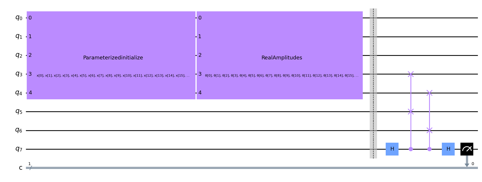
மீண்டும், swap சோதனையானது qubits \(3\), \(4\), \(5\) மற்றும் \(6\) ஆகியவற்றில் செய்யப்படுவதைக் காணலாம், இது நமது செலவுச் செயல்பாட்டின் மதிப்பைத் தீர்மானிக்கும்.
[15]:
def identity_interpret(x):
    return x


qnn = SamplerQNN(
    circuit=qc,
    input_params=fm.parameters,
    weight_params=ae.parameters,
    interpret=identity_interpret,
    output_shape=2,
)
We build our cost function, based on the swap test between the reference and trash space for the digit dataset. To do this, we again use Qiskit Machine Learning’s CircuitQNN network and use the same interpret function as we are measuring the probability of getting the final qubit in the \(|1\rangle\) state.
[16]:
def cost_func_digits(params_values):
    probabilities = qnn.forward(train_images, params_values)
    cost = np.sum(probabilities[:, 1]) / train_images.shape[0]

    # plotting part
    clear_output(wait=True)
    objective_func_vals.append(cost)
    plt.title("Objective function value against iteration")
    plt.xlabel("Iteration")
    plt.ylabel("Objective function value")
    plt.plot(range(len(objective_func_vals)), objective_func_vals)
    plt.show()

    return cost
Since model training may take a long time we have already pre-trained the model for some iterations and saved the pre-trained weights. We’ll continue training from that point by setting initial_point to a vector of pre-trained weights.
[17]:
with open("12_qae_initial_point.json", "r") as f:
    initial_point = json.load(f)
By minimizing this cost function, we can thus determine the required parameters to compress our noisy images. Let’s see if we can encode our images!
[18]:
opt = COBYLA(maxiter=150)

objective_func_vals = []
# make the plot nicer
plt.rcParams["figure.figsize"] = (12, 6)

start = time.time()
opt_result = opt.minimize(fun=cost_func_digits, x0=initial_point)
elapsed = time.time() - start
print(f"Fit in {elapsed:0.2f} seconds")
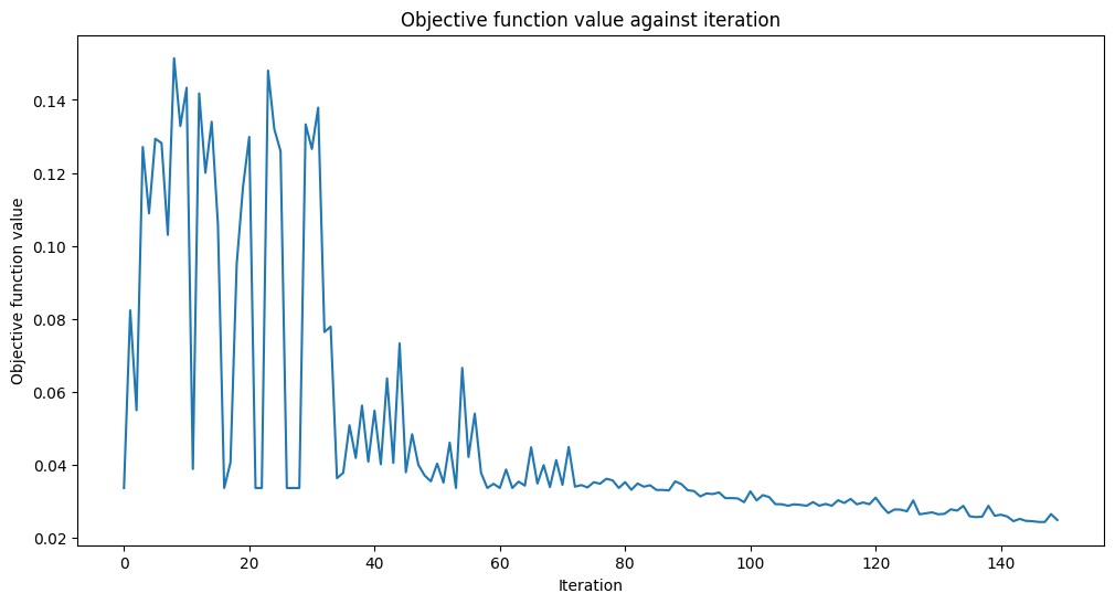
Fit in 40.59 seconds
அது ஒன்றிணைந்தது போல் தெரிகிறது!
Now let’s build our Encoder and Decoder using the parameters obtained from the training period. After applying this circuit to our new dataset, we can then compare our input and output data and see if we were able to retain the images efficiently throughout the compression!
[19]:
# Test
test_qc = QuantumCircuit(num_latent + num_trash)
test_qc = test_qc.compose(fm)
ansatz_qc = ansatz(num_latent + num_trash)
test_qc = test_qc.compose(ansatz_qc)
test_qc.barrier()
test_qc.reset(4)
test_qc.reset(3)
test_qc.barrier()
test_qc = test_qc.compose(ansatz_qc.inverse())

# sample new images
test_images, test_labels = get_dataset_digits(2, draw=False)
for image, label in zip(test_images, test_labels):
    original_qc = fm.assign_parameters(image)
    original_sv = Statevector(original_qc).data
    original_sv = np.reshape(np.abs(original_sv) ** 2, (8, 4))

    param_values = np.concatenate((image, opt_result.x))
    output_qc = test_qc.assign_parameters(param_values)
    output_sv = Statevector(output_qc).data
    output_sv = np.reshape(np.abs(output_sv) ** 2, (8, 4))

    fig, (ax1, ax2) = plt.subplots(1, 2)
    ax1.imshow(original_sv)
    ax1.set_title("Input Data")
    ax2.imshow(output_sv)
    ax2.set_title("Output Data")
    plt.show()
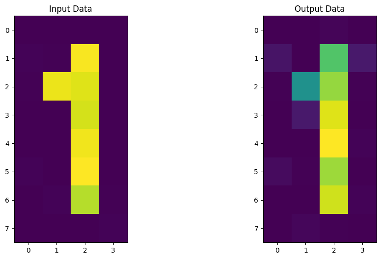
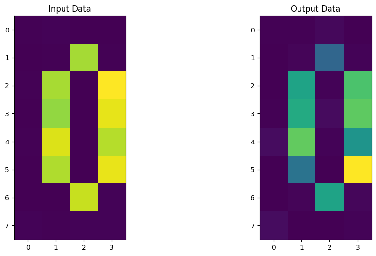
It looks like our Quantum Autoencoder can be trained to encode digits as well! Now it’s your turn to build your own Quantum Autoencoder and come up with ideas and datasets to compress!
8. குவாண்டம் ஆட்டோஎன்கோடரின் பயன்பாடுகள்#
Quantum Autoencoder’s can be used for various different applications, including
டிஜிட்டல் சுருக்கம்: தகவல் சிறிய அளவு குவிட்களில் குறியாக்கம் செய்யப்படலாம். குவாண்டம் சாதனங்களுக்கு இது மிகவும் பயனுள்ளதாக இருக்கும், ஏனெனில் சிறிய குவிட் அமைப்புகள் சத்தத்திற்கு ஆளாகின்றன.
Denoising: குவாண்டம் ஆட்டோஎன்கோடரைப் பயன்படுத்தி, ஆரம்ப குவாண்டம் நிலை அல்லது குறியிடப்பட்ட தரவிலிருந்து தொடர்புடைய அம்சங்களைப் பிரித்தெடுக்கலாம், அதே நேரத்தில் கூடுதல் சத்தத்தைப் புறக்கணிக்கலாம்.
குவாண்டம் வேதியியல்: இதில் குவாண்டம் ஆட்டோஎன்கோடரை ஹப்பார்ட் மாடல் போன்ற அமைப்புகளுக்கு அன்சாட்ஸாகப் பயன்படுத்தலாம். இது பொதுவாக மூலக்கூறுகளில் எலக்ட்ரான்-எலக்ட்ரான் தொடர்புகளை விவரிக்கப் பயன்படுகிறது.
9. குறிப்புகள்#
ஆட்டோஎன்கோடரில் ஒரு விக்கிபீடியா பக்கம்: https://en.wikipedia.org/wiki/Autoencoder
Romero, Jonathan, Jonathan P. Olson, and Alan Aspuru-Guzik. "Quantum autoencoders for efficient compression of quantum data." Quantum Science and Technology 2.4 (2017): 045001.
ஸ்வாப் டெஸ்ட் அல்காரிதம்: https://en.wikipedia.org/wiki/Swap_test
[20]:
import qiskit.tools.jupyter

%qiskit_version_table
%qiskit_copyright
Version Information
| Qiskit Software | Version |
|---|---|
qiskit-terra | 0.22.2 |
qiskit-aer | 0.11.1 |
qiskit-machine-learning | 0.6.0 |
| System information | |
| Python version | 3.8.13 |
| Python compiler | Clang 12.0.0 |
| Python build | default, Oct 19 2022 17:54:22 |
| OS | Darwin |
| CPUs | 10 |
| Memory (Gb) | 64.0 |
| Thu Nov 10 23:26:05 2022 GMT | |
This code is a part of Qiskit
© Copyright IBM 2017, 2022.
This code is licensed under the Apache License, Version 2.0. You may
obtain a copy of this license in the LICENSE.txt file in the root directory
of this source tree or at http://www.apache.org/licenses/LICENSE-2.0.
Any modifications or derivative works of this code must retain this
copyright notice, and modified files need to carry a notice indicating
that they have been altered from the originals.