참고
이 페이지는 docs/tutorials/05_torch_connector.ipynb 에서 생성되었다.
토치 커넥터 및 하이브리드 QNN#
This tutorial introduces the TorchConnector class, and demonstrates how it allows for a natural integration of any NeuralNetwork from Qiskit Machine Learning into a PyTorch workflow. TorchConnector takes a NeuralNetwork and makes it available as a PyTorch Module. The resulting module can be seamlessly incorporated into PyTorch classical architectures and trained jointly without additional considerations, enabling the development and testing of novel hybrid
quantum-classical machine learning architectures.
내용:#
파트 1: 단순 분류 및 회귀
The first part of this tutorial shows how quantum neural networks can be trained using PyTorch’s automatic differentiation engine (torch.autograd, link) for simple classification and regression tasks.
분류
Classification with PyTorch and
EstimatorQNNClassification with PyTorch and
SamplerQNN
회귀
Regression with PyTorch and
EstimatorQNN
Part 2: MNIST 분류, 하이브리드 QNN
이 튜토리얼의 두 번째 부분에서는 하이브리드 양자-고전 방식으로 MNIST 데이터를 분류하기 위해 (이 경우에는 전형적인 CNN 아키텍처인) 대상 PyTorch 워크플로에 (양자) NeuralNetwork 를 삽입하는 방법을 설명한다.
[1]:
# Necessary imports

import numpy as np
import matplotlib.pyplot as plt

from torch import Tensor
from torch.nn import Linear, CrossEntropyLoss, MSELoss
from torch.optim import LBFGS

from qiskit import QuantumCircuit
from qiskit.circuit import Parameter
from qiskit.circuit.library import RealAmplitudes, ZZFeatureMap
from qiskit_algorithms.utils import algorithm_globals
from qiskit_machine_learning.neural_networks import SamplerQNN, EstimatorQNN
from qiskit_machine_learning.connectors import TorchConnector

# Set seed for random generators
algorithm_globals.random_seed = 42
파트 1: 단순 분류 및 회귀#
1. 분류#
First, we show how TorchConnector allows to train a Quantum NeuralNetwork to solve a classification tasks using PyTorch’s automatic differentiation engine. In order to illustrate this, we will perform binary classification on a randomly generated dataset.
[2]:
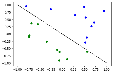
# Generate random dataset

# Select dataset dimension (num_inputs) and size (num_samples)
num_inputs = 2
num_samples = 20

# Generate random input coordinates (X) and binary labels (y)
X = 2 * algorithm_globals.random.random([num_samples, num_inputs]) - 1
y01 = 1 * (np.sum(X, axis=1) >= 0)  # in { 0,  1}, y01 will be used for SamplerQNN example
y = 2 * y01 - 1  # in {-1, +1}, y will be used for EstimatorQNN example

# Convert to torch Tensors
X_ = Tensor(X)
y01_ = Tensor(y01).reshape(len(y)).long()
y_ = Tensor(y).reshape(len(y), 1)

# Plot dataset
for x, y_target in zip(X, y):
    if y_target == 1:
        plt.plot(x[0], x[1], "bo")
    else:
        plt.plot(x[0], x[1], "go")
plt.plot([-1, 1], [1, -1], "--", color="black")
plt.show()
A. Classification with PyTorch and EstimatorQNN#
Linking an EstimatorQNN to PyTorch is relatively straightforward. Here we illustrate this by using the EstimatorQNN constructed from a feature map and an ansatz.
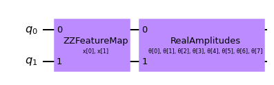
[3]:
# Set up a circuit
feature_map = ZZFeatureMap(num_inputs)
ansatz = RealAmplitudes(num_inputs)
qc = QuantumCircuit(num_inputs)
qc.compose(feature_map, inplace=True)
qc.compose(ansatz, inplace=True)
qc.draw("mpl")
[3]:
[4]:
# Setup QNN
qnn1 = EstimatorQNN(
    circuit=qc, input_params=feature_map.parameters, weight_params=ansatz.parameters
)

# Set up PyTorch module
# Note: If we don't explicitly declare the initial weights
# they are chosen uniformly at random from [-1, 1].
initial_weights = 0.1 * (2 * algorithm_globals.random.random(qnn1.num_weights) - 1)
model1 = TorchConnector(qnn1, initial_weights=initial_weights)
print("Initial weights: ", initial_weights)
Initial weights:  [-0.01256962  0.06653564  0.04005302 -0.03752667  0.06645196  0.06095287
 -0.02250432 -0.04233438]
[5]:
# Test with a single input
model1(X_[0, :])
[5]:
tensor([-0.3285], grad_fn=<_TorchNNFunctionBackward>)
최적화 도구#
The choice of optimizer for training any machine learning model can be crucial in determining the success of our training’s outcome. When using TorchConnector, we get access to all of the optimizer algorithms defined in the [torch.optim] package (link). Some of the most famous algorithms used in popular machine learning architectures include Adam, SGD, or Adagrad. However, for this tutorial we will be using the L-BFGS algorithm
(torch.optim.LBFGS), one of the most well know second-order optimization algorithms for numerical optimization.
손실 함수#
As for the loss function, we can also take advantage of PyTorch’s pre-defined modules from torch.nn, such as the Cross-Entropy or Mean Squared Error losses.
💡 Clarification : In classical machine learning, the general rule of thumb is to apply a Cross-Entropy loss to classification tasks, and MSE loss to regression tasks. However, this recommendation is given under the assumption that the output of the classification network is a class probability value in the EstimatorQNN does not include such layer, and we don’t apply any mapping to
the output (the following section shows an example of application of parity mapping with SamplerQNNs), the QNN’s output can take any value in the range
[6]:
# Define optimizer and loss
optimizer = LBFGS(model1.parameters())
f_loss = MSELoss(reduction="sum")

# Start training
model1.train()  # set model to training mode


# Note from (https://pytorch.org/docs/stable/optim.html):
# Some optimization algorithms such as LBFGS need to
# reevaluate the function multiple times, so you have to
# pass in a closure that allows them to recompute your model.
# The closure should clear the gradients, compute the loss,
# and return it.
def closure():
    optimizer.zero_grad()  # Initialize/clear gradients
    loss = f_loss(model1(X_), y_)  # Evaluate loss function
    loss.backward()  # Backward pass
    print(loss.item())  # Print loss
    return loss


# Run optimizer step4
optimizer.step(closure)
25.535646438598633
22.696760177612305
20.039228439331055
19.687908172607422
19.267208099365234
19.025373458862305
18.154708862304688
17.337854385375977
19.082578659057617
17.073287963867188
16.21839141845703
14.992582321166992
14.929339408874512
14.914533615112305
14.907636642456055
14.902364730834961
14.902134895324707
14.90211009979248
14.902111053466797
[6]:
tensor(25.5356, grad_fn=<MseLossBackward0>)
[7]:
# Evaluate model and compute accuracy
model1.eval()
y_predict = []
for x, y_target in zip(X, y):
    output = model1(Tensor(x))
    y_predict += [np.sign(output.detach().numpy())[0]]

print("Accuracy:", sum(y_predict == y) / len(y))

# Plot results
# red == wrongly classified
for x, y_target, y_p in zip(X, y, y_predict):
    if y_target == 1:
        plt.plot(x[0], x[1], "bo")
    else:
        plt.plot(x[0], x[1], "go")
    if y_target != y_p:
        plt.scatter(x[0], x[1], s=200, facecolors="none", edgecolors="r", linewidths=2)
plt.plot([-1, 1], [1, -1], "--", color="black")
plt.show()
Accuracy: 0.8
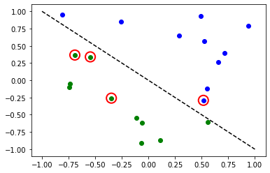
빨간색 원은 잘못 분류된 데이터 포인트들을 나타낸다.
B. Classification with PyTorch and SamplerQNN#
Linking a SamplerQNN to PyTorch requires a bit more attention than EstimatorQNN. Without the correct setup, backpropagation is not possible.
In particular, we must make sure that we are returning a dense array of probabilities in the network’s forward pass (sparse=False). This parameter is set up to False by default, so we just have to make sure that it has not been changed.
⚠️ Attention: If we define a custom interpret function ( in the example: parity), we must remember to explicitly provide the desired output shape ( in the example: 2). For more info on the initial parameter setup for SamplerQNN, please check out the official qiskit documentation.
[8]:
# Define feature map and ansatz
feature_map = ZZFeatureMap(num_inputs)
ansatz = RealAmplitudes(num_inputs, entanglement="linear", reps=1)

# Define quantum circuit of num_qubits = input dim
# Append feature map and ansatz
qc = QuantumCircuit(num_inputs)
qc.compose(feature_map, inplace=True)
qc.compose(ansatz, inplace=True)

# Define SamplerQNN and initial setup
parity = lambda x: "{:b}".format(x).count("1") % 2  # optional interpret function
output_shape = 2  # parity = 0, 1
qnn2 = SamplerQNN(
    circuit=qc,
    input_params=feature_map.parameters,
    weight_params=ansatz.parameters,
    interpret=parity,
    output_shape=output_shape,
)

# Set up PyTorch module
# Reminder: If we don't explicitly declare the initial weights
# they are chosen uniformly at random from [-1, 1].
initial_weights = 0.1 * (2 * algorithm_globals.random.random(qnn2.num_weights) - 1)
print("Initial weights: ", initial_weights)
model2 = TorchConnector(qnn2, initial_weights)
Initial weights: [ 0.0364991 -0.0720495 -0.06001836 -0.09852755]
최적화 함수 및 손실 함수에 대한 자세한 사항은 최적화 함수 를 통해 확인할 수 있다.
[9]:
# Define model, optimizer, and loss
optimizer = LBFGS(model2.parameters())
f_loss = CrossEntropyLoss()  # Our output will be in the [0,1] range

# Start training
model2.train()

# Define LBFGS closure method (explained in previous section)
def closure():
    optimizer.zero_grad(set_to_none=True)  # Initialize gradient
    loss = f_loss(model2(X_), y01_)  # Calculate loss
    loss.backward()  # Backward pass

    print(loss.item())  # Print loss
    return loss


# Run optimizer (LBFGS requires closure)
optimizer.step(closure);
0.6925069093704224
0.6881508231163025
0.6516683101654053
0.6485998034477234
0.6394743919372559
0.7057444453239441
0.669085681438446
0.766187310218811
0.7188469171524048
0.7919709086418152
0.7598814964294434
0.7028256058692932
0.7486447095870972
0.6890242695808411
0.7760348916053772
0.7892935276031494
0.7556288242340088
0.7058126330375671
0.7203161716461182
0.7030722498893738
[10]:
# Evaluate model and compute accuracy
model2.eval()
y_predict = []
for x in X:
    output = model2(Tensor(x))
    y_predict += [np.argmax(output.detach().numpy())]

print("Accuracy:", sum(y_predict == y01) / len(y01))

# plot results
# red == wrongly classified
for x, y_target, y_ in zip(X, y01, y_predict):
    if y_target == 1:
        plt.plot(x[0], x[1], "bo")
    else:
        plt.plot(x[0], x[1], "go")
    if y_target != y_:
        plt.scatter(x[0], x[1], s=200, facecolors="none", edgecolors="r", linewidths=2)
plt.plot([-1, 1], [1, -1], "--", color="black")
plt.show()
Accuracy: 0.5
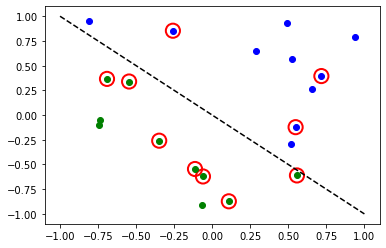
빨간색 원은 잘못 분류된 데이터 포인트들을 나타낸다.
2. 회귀#
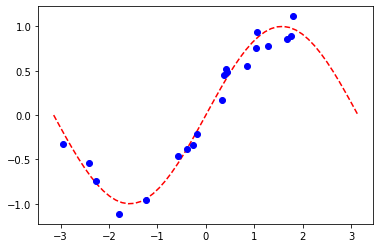
We use a model based on the EstimatorQNN to also illustrate how to perform a regression task. The chosen dataset in this case is randomly generated following a sine wave.
[11]:
# Generate random dataset

num_samples = 20
eps = 0.2
lb, ub = -np.pi, np.pi
f = lambda x: np.sin(x)

X = (ub - lb) * algorithm_globals.random.random([num_samples, 1]) + lb
y = f(X) + eps * (2 * algorithm_globals.random.random([num_samples, 1]) - 1)
plt.plot(np.linspace(lb, ub), f(np.linspace(lb, ub)), "r--")
plt.plot(X, y, "bo")
plt.show()
A. Regression with PyTorch and EstimatorQNN#
The network definition and training loop will be analogous to those of the classification task using EstimatorQNN. In this case, we define our own feature map and ansatz, but let’s do it a little different.
[12]:
# Construct simple feature map
param_x = Parameter("x")
feature_map = QuantumCircuit(1, name="fm")
feature_map.ry(param_x, 0)

# Construct simple parameterized ansatz
param_y = Parameter("y")
ansatz = QuantumCircuit(1, name="vf")
ansatz.ry(param_y, 0)

qc = QuantumCircuit(1)
qc.compose(feature_map, inplace=True)
qc.compose(ansatz, inplace=True)

# Construct QNN
qnn3 = EstimatorQNN(circuit=qc, input_params=[param_x], weight_params=[param_y])

# Set up PyTorch module
# Reminder: If we don't explicitly declare the initial weights
# they are chosen uniformly at random from [-1, 1].
initial_weights = 0.1 * (2 * algorithm_globals.random.random(qnn3.num_weights) - 1)
model3 = TorchConnector(qnn3, initial_weights)
최적화 함수 및 손실 함수에 대한 자세한 사항은 최적화 함수 를 통해 확인할 수 있다.
[13]:
# Define optimizer and loss function
optimizer = LBFGS(model3.parameters())
f_loss = MSELoss(reduction="sum")

# Start training
model3.train()  # set model to training mode

# Define objective function
def closure():
    optimizer.zero_grad(set_to_none=True)  # Initialize gradient
    loss = f_loss(model3(Tensor(X)), Tensor(y))  # Compute batch loss
    loss.backward()  # Backward pass
    print(loss.item())  # Print loss
    return loss


# Run optimizer
optimizer.step(closure)
14.947757720947266
2.948650360107422
8.952412605285645
0.37905153632164
0.24995625019073486
0.2483610212802887
0.24835753440856934
[13]:
tensor(14.9478, grad_fn=<MseLossBackward0>)
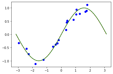
[14]:
# Plot target function
plt.plot(np.linspace(lb, ub), f(np.linspace(lb, ub)), "r--")

# Plot data
plt.plot(X, y, "bo")

# Plot fitted line
model3.eval()
y_ = []
for x in np.linspace(lb, ub):
    output = model3(Tensor([x]))
    y_ += [output.detach().numpy()[0]]
plt.plot(np.linspace(lb, ub), y_, "g-")
plt.show()
파트 2: MNIST 분류, 하이브리드 QNN#
이 두 번째 부분에서는 TorchConnector 를 사용하여 하이브리드 양자-고전 신경망을 활용하여 MNIST 자필 숫자 데이터 셋에 보다 복잡한 이미지 분류 작업을 수행하는 방법을 설명한다.
하이브리드 양자-고전 신경망에 대한 보다 자세한 설명 (pre-TorchConnector) 에 대해서는 `Qiskit Textbook <https://qiskit.org/textbook/ch-machine-learning/machine-learning-qiskit-pytorch.html>`__의 해당 섹션을 확인할 수 있다.
[15]:
# Additional torch-related imports
import torch
from torch import cat, no_grad, manual_seed
from torch.utils.data import DataLoader
from torchvision import datasets, transforms
import torch.optim as optim
from torch.nn import (
    Module,
    Conv2d,
    Linear,
    Dropout2d,
    NLLLoss,
    MaxPool2d,
    Flatten,
    Sequential,
    ReLU,
)
import torch.nn.functional as F
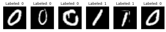
1단계: 훈련 및 테스트를 위한 데이터 로더 정의#
우리는 torchvision API 를 이용하여 MNIST dataset 의 서브셋을 직접 로드하고, torch DataLoaders (link)를 훈련과 테스트에 사용할 수 있도록 한다.
[16]:
# Train Dataset
# -------------

# Set train shuffle seed (for reproducibility)
manual_seed(42)

batch_size = 1
n_samples = 100  # We will concentrate on the first 100 samples

# Use pre-defined torchvision function to load MNIST train data
X_train = datasets.MNIST(
    root="./data", train=True, download=True, transform=transforms.Compose([transforms.ToTensor()])
)

# Filter out labels (originally 0-9), leaving only labels 0 and 1
idx = np.append(
    np.where(X_train.targets == 0)[0][:n_samples], np.where(X_train.targets == 1)[0][:n_samples]
)
X_train.data = X_train.data[idx]
X_train.targets = X_train.targets[idx]

# Define torch dataloader with filtered data
train_loader = DataLoader(X_train, batch_size=batch_size, shuffle=True)
빠른 시각화를 수행하는 경우 훈련 데이터 셋이 손으로 쓴 0과 1의 이미지로 구성되어 있음을 알 수 있다.
[17]:
n_samples_show = 6

data_iter = iter(train_loader)
fig, axes = plt.subplots(nrows=1, ncols=n_samples_show, figsize=(10, 3))

while n_samples_show > 0:
    images, targets = data_iter.__next__()

    axes[n_samples_show - 1].imshow(images[0, 0].numpy().squeeze(), cmap="gray")
    axes[n_samples_show - 1].set_xticks([])
    axes[n_samples_show - 1].set_yticks([])
    axes[n_samples_show - 1].set_title("Labeled: {}".format(targets[0].item()))

    n_samples_show -= 1
[18]:
# Test Dataset
# -------------

# Set test shuffle seed (for reproducibility)
# manual_seed(5)

n_samples = 50

# Use pre-defined torchvision function to load MNIST test data
X_test = datasets.MNIST(
    root="./data", train=False, download=True, transform=transforms.Compose([transforms.ToTensor()])
)

# Filter out labels (originally 0-9), leaving only labels 0 and 1
idx = np.append(
    np.where(X_test.targets == 0)[0][:n_samples], np.where(X_test.targets == 1)[0][:n_samples]
)
X_test.data = X_test.data[idx]
X_test.targets = X_test.targets[idx]

# Define torch dataloader with filtered data
test_loader = DataLoader(X_test, batch_size=batch_size, shuffle=True)
단계 2: QNN및 하이브리드 모델 정의#
This second step shows the power of the TorchConnector. After defining our quantum neural network layer (in this case, a EstimatorQNN), we can embed it into a layer in our torch Module by initializing a torch connector as TorchConnector(qnn).
⚠️ 주의: 하이브리드 모델에서 적절한 그라디언트 역전파를 수행하려면 qnn 초기화 중에 초기 매개변수 input_gradients 를 TRUE로 설정해야 한다.
[19]:
# Define and create QNN
def create_qnn():
    feature_map = ZZFeatureMap(2)
    ansatz = RealAmplitudes(2, reps=1)
    qc = QuantumCircuit(2)
    qc.compose(feature_map, inplace=True)
    qc.compose(ansatz, inplace=True)

    # REMEMBER TO SET input_gradients=True FOR ENABLING HYBRID GRADIENT BACKPROP
    qnn = EstimatorQNN(
        circuit=qc,
        input_params=feature_map.parameters,
        weight_params=ansatz.parameters,
        input_gradients=True,
    )
    return qnn


qnn4 = create_qnn()
[20]:
# Define torch NN module


class Net(Module):
    def __init__(self, qnn):
        super().__init__()
        self.conv1 = Conv2d(1, 2, kernel_size=5)
        self.conv2 = Conv2d(2, 16, kernel_size=5)
        self.dropout = Dropout2d()
        self.fc1 = Linear(256, 64)
        self.fc2 = Linear(64, 2)  # 2-dimensional input to QNN
        self.qnn = TorchConnector(qnn)  # Apply torch connector, weights chosen
        # uniformly at random from interval [-1,1].
        self.fc3 = Linear(1, 1)  # 1-dimensional output from QNN

    def forward(self, x):
        x = F.relu(self.conv1(x))
        x = F.max_pool2d(x, 2)
        x = F.relu(self.conv2(x))
        x = F.max_pool2d(x, 2)
        x = self.dropout(x)
        x = x.view(x.shape[0], -1)
        x = F.relu(self.fc1(x))
        x = self.fc2(x)
        x = self.qnn(x)  # apply QNN
        x = self.fc3(x)
        return cat((x, 1 - x), -1)


model4 = Net(qnn4)
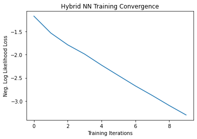
단계 3: 훈련#
[21]:
# Define model, optimizer, and loss function
optimizer = optim.Adam(model4.parameters(), lr=0.001)
loss_func = NLLLoss()

# Start training
epochs = 10  # Set number of epochs
loss_list = []  # Store loss history
model4.train()  # Set model to training mode

for epoch in range(epochs):
    total_loss = []
    for batch_idx, (data, target) in enumerate(train_loader):
        optimizer.zero_grad(set_to_none=True)  # Initialize gradient
        output = model4(data)  # Forward pass
        loss = loss_func(output, target)  # Calculate loss
        loss.backward()  # Backward pass
        optimizer.step()  # Optimize weights
        total_loss.append(loss.item())  # Store loss
    loss_list.append(sum(total_loss) / len(total_loss))
    print("Training [{:.0f}%]\tLoss: {:.4f}".format(100.0 * (epoch + 1) / epochs, loss_list[-1]))
Training [10%]  Loss: -1.1630
Training [20%]  Loss: -1.5294
Training [30%]  Loss: -1.7855
Training [40%]  Loss: -1.9863
Training [50%]  Loss: -2.2257
Training [60%]  Loss: -2.4513
Training [70%]  Loss: -2.6758
Training [80%]  Loss: -2.8832
Training [90%]  Loss: -3.1006
Training [100%] Loss: -3.3061
[22]:
# Plot loss convergence
plt.plot(loss_list)
plt.title("Hybrid NN Training Convergence")
plt.xlabel("Training Iterations")
plt.ylabel("Neg. Log Likelihood Loss")
plt.show()
Now we’ll save the trained model, just to show how a hybrid model can be saved and re-used later for inference. To save and load hybrid models, when using the TorchConnector, follow the PyTorch recommendations of saving and loading the models.
[23]:
torch.save(model4.state_dict(), "model4.pt")
단계 4: 평가#
모델을 다시 생성하고 이전에 저장된 파일에서 상태를 불러오는 것부터 시작한다. 다른 시뮬레이터나 실제 하드웨어로 QNN 계층을 만든다. 그리고 클라우드에서 사용할 수 있는 실제 하드웨어에서 모델을 훈련시키고 추론은 시뮬레이터로 하거나 또는 반대로 할 수도 있다. 간단하게, 위와 같이 새로운 양자 신경망을 만든다.
[24]:
qnn5 = create_qnn()
model5 = Net(qnn5)
model5.load_state_dict(torch.load("model4.pt"))
[24]:
<All keys matched successfully>
[25]:
model5.eval()  # set model to evaluation mode
with no_grad():

    correct = 0
    for batch_idx, (data, target) in enumerate(test_loader):
        output = model5(data)
        if len(output.shape) == 1:
            output = output.reshape(1, *output.shape)

        pred = output.argmax(dim=1, keepdim=True)
        correct += pred.eq(target.view_as(pred)).sum().item()

        loss = loss_func(output, target)
        total_loss.append(loss.item())

    print(
        "Performance on test data:\n\tLoss: {:.4f}\n\tAccuracy: {:.1f}%".format(
            sum(total_loss) / len(total_loss), correct / len(test_loader) / batch_size * 100
        )
    )
Performance on test data:
        Loss: -3.3585
        Accuracy: 100.0%
[26]:
# Plot predicted labels

n_samples_show = 6
count = 0
fig, axes = plt.subplots(nrows=1, ncols=n_samples_show, figsize=(10, 3))

model5.eval()
with no_grad():
    for batch_idx, (data, target) in enumerate(test_loader):
        if count == n_samples_show:
            break
        output = model5(data[0:1])
        if len(output.shape) == 1:
            output = output.reshape(1, *output.shape)

        pred = output.argmax(dim=1, keepdim=True)

        axes[count].imshow(data[0].numpy().squeeze(), cmap="gray")

        axes[count].set_xticks([])
        axes[count].set_yticks([])
        axes[count].set_title("Predicted {}".format(pred.item()))

        count += 1
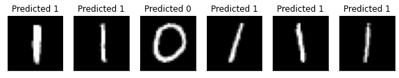
🎉🎉🎉🎉 이제 Qiskit Machine Learning을 사용하여 자체 하이브리드 데이터 세트 및 아키텍처를 실험할 수 있다. ** **행운을 빈다!
[27]:
import qiskit.tools.jupyter

%qiskit_version_table
%qiskit_copyright
Version Information
| Qiskit Software | Version |
|---|---|
qiskit-terra | 0.22.0 |
qiskit-aer | 0.11.1 |
qiskit-ignis | 0.7.0 |
qiskit | 0.33.0 |
qiskit-machine-learning | 0.5.0 |
| System information | |
| Python version | 3.7.9 |
| Python compiler | MSC v.1916 64 bit (AMD64) |
| Python build | default, Aug 31 2020 17:10:11 |
| OS | Windows |
| CPUs | 4 |
| Memory (Gb) | 31.837730407714844 |
| Thu Nov 03 09:57:38 2022 GMT Standard Time | |
This code is a part of Qiskit
© Copyright IBM 2017, 2022.
This code is licensed under the Apache License, Version 2.0. You may
obtain a copy of this license in the LICENSE.txt file in the root directory
of this source tree or at http://www.apache.org/licenses/LICENSE-2.0.
Any modifications or derivative works of this code must retain this
copyright notice, and modified files need to carry a notice indicating
that they have been altered from the originals.