참고
이 페이지는 docs/tutorials/02_neural_network_classifier_and_regressor.ipynb 에서 생성되었다.
신경망 분류기 & 회귀기#
이 튜토리얼에서는 NeuralNetworkClassifier 와 NeuralNetworkRegressor 가 어떻게 사용되는지를 보여준다. 두 가지 모두 (양자) NeuralNetwork 을 입력하고 이를 특정한 문맥에서 활용한다. 두 가지 모두 편의상 사전 구성된 Variational Quantum Classifier (VQC) 와 Variational Quantum Regressor (VQR) 도 제공한다. 이 튜토리얼은 다음과 같이 구성된다.
분류
Classification with an
EstimatorQNNClassification with a
SamplerQNN변분 양자분류기 (
VQC, Variational Quantum Classifier)
회귀
Regression with an
EstimatorQNN변분 양자회귀기 (
VQR, Variational Quantum Regressor)
[1]:
import matplotlib.pyplot as plt
import numpy as np
from IPython.display import clear_output
from qiskit import QuantumCircuit
from qiskit.circuit import Parameter
from qiskit.circuit.library import RealAmplitudes, ZZFeatureMap
from qiskit_algorithms.optimizers import COBYLA, L_BFGS_B
from qiskit_algorithms.utils import algorithm_globals

from qiskit_machine_learning.algorithms.classifiers import NeuralNetworkClassifier, VQC
from qiskit_machine_learning.algorithms.regressors import NeuralNetworkRegressor, VQR
from qiskit_machine_learning.neural_networks import SamplerQNN, EstimatorQNN
from qiskit_machine_learning.circuit.library import QNNCircuit

algorithm_globals.random_seed = 42
분류#
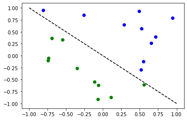
다음 알고리즘을 설명하기 위해 간단한 분류 데이터 셋을 준비한다.
[2]:
num_inputs = 2
num_samples = 20
X = 2 * algorithm_globals.random.random([num_samples, num_inputs]) - 1
y01 = 1 * (np.sum(X, axis=1) >= 0)  # in { 0,  1}
y = 2 * y01 - 1  # in {-1, +1}
y_one_hot = np.zeros((num_samples, 2))
for i in range(num_samples):
    y_one_hot[i, y01[i]] = 1

for x, y_target in zip(X, y):
    if y_target == 1:
        plt.plot(x[0], x[1], "bo")
    else:
        plt.plot(x[0], x[1], "go")
plt.plot([-1, 1], [1, -1], "--", color="black")
plt.show()
Classification with an EstimatorQNN#
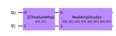
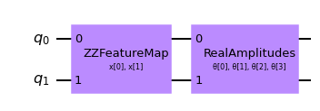
First we show how an EstimatorQNN can be used for classification within a NeuralNetworkClassifier. In this context, the EstimatorQNN is expected to return one-dimensional output in \([-1, +1]\). This only works for binary classification and we assign the two classes to \(\{-1, +1\}\). To simplify the composition of parameterized quantum circuit from a feature map and an ansatz we can use the QNNCircuit class.
[3]:
# construct QNN with the QNNCircuit's default ZZFeatureMap feature map and RealAmplitudes ansatz.
qc = QNNCircuit(num_qubits=2)
qc.draw(output="mpl")
[3]:
Create a quantum neural network
[4]:
estimator_qnn = EstimatorQNN(circuit=qc)
[5]:
# QNN maps inputs to [-1, +1]
estimator_qnn.forward(X[0, :], algorithm_globals.random.random(estimator_qnn.num_weights))
[5]:
array([[0.23521988]])
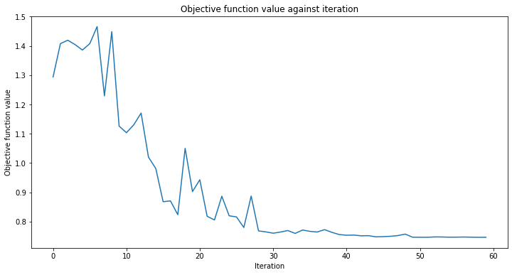
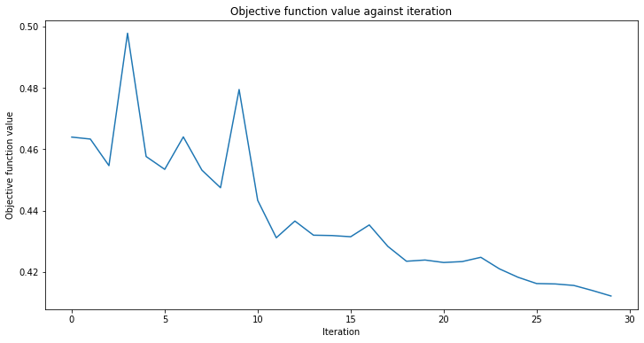
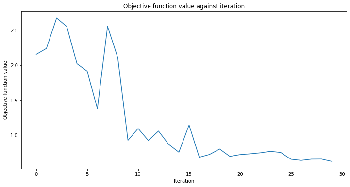
callback_graph 라는 콜백 함수를 추가할 것이다. 이 함수는 최적화 단계가 반복될 때마다 호출되며 두 개의 매개변수(현재 가중치와 해당 가중치에 대한 최적화 시키려는 목적 함수의 값)가 전달된다. 목적 함수의 값을 배열에 추가함으로써 반복 횟수 대비 목적 함수의 값을 그래프로 출력하고 반복적으로 해당 그래프를 갱신할 수 있게 한다. 그러나 이 외에도 콜백 함수 및 함수로 전달되는 두 개의 매개변수를 이용해 원하는 동작은 무엇이든 할 수 있다.
[6]:
# callback function that draws a live plot when the .fit() method is called
def callback_graph(weights, obj_func_eval):
    clear_output(wait=True)
    objective_func_vals.append(obj_func_eval)
    plt.title("Objective function value against iteration")
    plt.xlabel("Iteration")
    plt.ylabel("Objective function value")
    plt.plot(range(len(objective_func_vals)), objective_func_vals)
    plt.show()
[7]:
# construct neural network classifier
estimator_classifier = NeuralNetworkClassifier(
    estimator_qnn, optimizer=COBYLA(maxiter=60), callback=callback_graph
)
[8]:
# create empty array for callback to store evaluations of the objective function
objective_func_vals = []
plt.rcParams["figure.figsize"] = (12, 6)

# fit classifier to data
estimator_classifier.fit(X, y)

# return to default figsize
plt.rcParams["figure.figsize"] = (6, 4)

# score classifier
estimator_classifier.score(X, y)
[8]:
0.8
[9]:
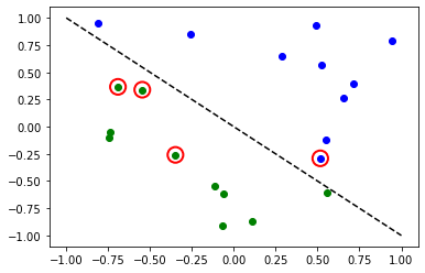
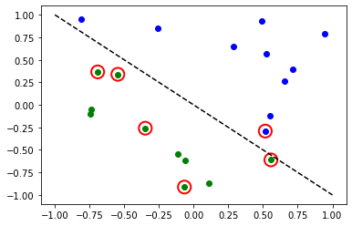
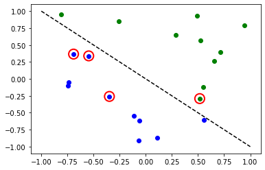
# evaluate data points
y_predict = estimator_classifier.predict(X)

# plot results
# red == wrongly classified
for x, y_target, y_p in zip(X, y, y_predict):
    if y_target == 1:
        plt.plot(x[0], x[1], "bo")
    else:
        plt.plot(x[0], x[1], "go")
    if y_target != y_p:
        plt.scatter(x[0], x[1], s=200, facecolors="none", edgecolors="r", linewidths=2)
plt.plot([-1, 1], [1, -1], "--", color="black")
plt.show()
Now, when the model is trained, we can explore the weights of the neural network. Please note, the number of weights is defined by ansatz.
[10]:
estimator_classifier.weights
[10]:
array([ 7.99142399e-01, -1.02869770e+00, -1.32131512e-04, -3.47046684e-01,
        1.13636802e+00,  6.56831727e-01,  2.17902158e+00, -1.08678332e+00])
Classification with a SamplerQNN#
Next we show how a SamplerQNN can be used for classification within a NeuralNetworkClassifier. In this context, the SamplerQNN is expected to return \(d\)-dimensional probability vector as output, where \(d\) denotes the number of classes. The underlying Sampler primitive returns quasi-distributions of bit strings and we just need to define a mapping from the measured bitstrings to the different classes. For binary classification we use the parity mapping. Again we can
use the QNNCircuit class to set up a parameterized quantum circuit from a feature map and ansatz of our choice.
[11]:
# construct a quantum circuit from the default ZZFeatureMap feature map and a customized RealAmplitudes ansatz
qc = QNNCircuit(ansatz=RealAmplitudes(num_inputs, reps=1))
qc.draw(output="mpl")
[11]:
[12]:
# parity maps bitstrings to 0 or 1
def parity(x):
    return "{:b}".format(x).count("1") % 2


output_shape = 2  # corresponds to the number of classes, possible outcomes of the (parity) mapping.
[13]:
# construct QNN
sampler_qnn = SamplerQNN(
    circuit=qc,
    interpret=parity,
    output_shape=output_shape,
)
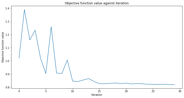
[14]:
# construct classifier
sampler_classifier = NeuralNetworkClassifier(
    neural_network=sampler_qnn, optimizer=COBYLA(maxiter=30), callback=callback_graph
)
[15]:
# create empty array for callback to store evaluations of the objective function
objective_func_vals = []
plt.rcParams["figure.figsize"] = (12, 6)

# fit classifier to data
sampler_classifier.fit(X, y01)

# return to default figsize
plt.rcParams["figure.figsize"] = (6, 4)

# score classifier
sampler_classifier.score(X, y01)
[15]:
0.7
[16]:
# evaluate data points
y_predict = sampler_classifier.predict(X)

# plot results
# red == wrongly classified
for x, y_target, y_p in zip(X, y01, y_predict):
    if y_target == 1:
        plt.plot(x[0], x[1], "bo")
    else:
        plt.plot(x[0], x[1], "go")
    if y_target != y_p:
        plt.scatter(x[0], x[1], s=200, facecolors="none", edgecolors="r", linewidths=2)
plt.plot([-1, 1], [1, -1], "--", color="black")
plt.show()
Again, once the model is trained we can take a look at the weights. As we set reps=1 explicitly in our ansatz, we can see less parameters than in the previous model.
[17]:
sampler_classifier.weights
[17]:
array([ 1.67198565, 0.46045402, -0.93462862, -0.95266092])
변분 양자분류기 (VQC, Variational Quantum Classifier)#
The VQC is a special variant of the NeuralNetworkClassifier with a SamplerQNN. It applies a parity mapping (or extensions to multiple classes) to map from the bitstring to the classification, which results in a probability vector, which is interpreted as a one-hot encoded result. By default, it applies this the CrossEntropyLoss function that expects labels given in one-hot encoded format and will return predictions in that format too.
[18]:
# construct feature map, ansatz, and optimizer
feature_map = ZZFeatureMap(num_inputs)
ansatz = RealAmplitudes(num_inputs, reps=1)

# construct variational quantum classifier
vqc = VQC(
    feature_map=feature_map,
    ansatz=ansatz,
    loss="cross_entropy",
    optimizer=COBYLA(maxiter=30),
    callback=callback_graph,
)
[19]:
# create empty array for callback to store evaluations of the objective function
objective_func_vals = []
plt.rcParams["figure.figsize"] = (12, 6)

# fit classifier to data
vqc.fit(X, y_one_hot)

# return to default figsize
plt.rcParams["figure.figsize"] = (6, 4)

# score classifier
vqc.score(X, y_one_hot)
[19]:
0.8
[20]:
# evaluate data points
y_predict = vqc.predict(X)

# plot results
# red == wrongly classified
for x, y_target, y_p in zip(X, y_one_hot, y_predict):
    if y_target[0] == 1:
        plt.plot(x[0], x[1], "bo")
    else:
        plt.plot(x[0], x[1], "go")
    if not np.all(y_target == y_p):
        plt.scatter(x[0], x[1], s=200, facecolors="none", edgecolors="r", linewidths=2)
plt.plot([-1, 1], [1, -1], "--", color="black")
plt.show()
Multiple classes with VQC#
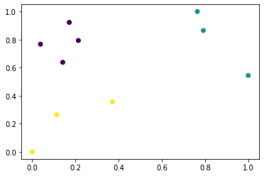
In this section we generate an artificial dataset that contains samples of three classes and show how to train a model to classify this dataset. This example shows how to tackle more interesting problems in machine learning. Of course, for a sake of short training time we prepare a tiny dataset. We employ make_classification from SciKit-Learn to generate a dataset. There 10 samples in the dataset, 2 features, that means we can still have a nice plot of the dataset, as well as no redundant
features, these are features are generated as a combinations of the other features. Also, we have 3 different classes in the dataset, each classes one kind of centroid and we set class separation to 2.0, a slight increase from the default value of 1.0 to ease the classification problem.
Once the dataset is generated we scale the features into the range [0, 1].
[21]:
from sklearn.datasets import make_classification
from sklearn.preprocessing import MinMaxScaler

X, y = make_classification(
    n_samples=10,
    n_features=2,
    n_classes=3,
    n_redundant=0,
    n_clusters_per_class=1,
    class_sep=2.0,
    random_state=algorithm_globals.random_seed,
)
X = MinMaxScaler().fit_transform(X)
Let’s see how our dataset looks like.
[22]:
plt.scatter(X[:, 0], X[:, 1], c=y)
[22]:
<matplotlib.collections.PathCollection at 0x7fd5e072c250>
We also transform labels and make them categorical.
[23]:
y_cat = np.empty(y.shape, dtype=str)
y_cat[y == 0] = "A"
y_cat[y == 1] = "B"
y_cat[y == 2] = "C"
print(y_cat)
['A' 'A' 'B' 'C' 'C' 'A' 'B' 'B' 'A' 'C']
We create an instance of VQC similar to the previous example, but in this case we pass a minimal set of parameters. Instead of feature map and ansatz we pass just the number of qubits that is equal to the number of features in the dataset, an optimizer with a low number of iteration to reduce training time, a quantum instance, and a callback to observe progress.
[24]:
vqc = VQC(
    num_qubits=2,
    optimizer=COBYLA(maxiter=30),
    callback=callback_graph,
)
Start the training process in the same way as in previous examples.
[25]:
# create empty array for callback to store evaluations of the objective function
objective_func_vals = []
plt.rcParams["figure.figsize"] = (12, 6)

# fit classifier to data
vqc.fit(X, y_cat)

# return to default figsize
plt.rcParams["figure.figsize"] = (6, 4)

# score classifier
vqc.score(X, y_cat)
[25]:
0.9
Despite we had the low number of iterations, we achieved quite a good score. Let see the output of the predict method and compare the output with the ground truth.
[26]:
predict = vqc.predict(X)
print(f"Predicted labels: {predict}")
print(f"Ground truth:     {y_cat}")
Predicted labels: ['A' 'A' 'B' 'C' 'C' 'A' 'B' 'B' 'A' 'B']
Ground truth:     ['A' 'A' 'B' 'C' 'C' 'A' 'B' 'B' 'A' 'C']
회귀#
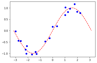
다음 알고리즘을 설명하기 위해 간단한 회귀 데이터셋을 준비한다.
[27]:
num_samples = 20
eps = 0.2
lb, ub = -np.pi, np.pi
X_ = np.linspace(lb, ub, num=50).reshape(50, 1)
f = lambda x: np.sin(x)

X = (ub - lb) * algorithm_globals.random.random([num_samples, 1]) + lb
y = f(X[:, 0]) + eps * (2 * algorithm_globals.random.random(num_samples) - 1)

plt.plot(X_, f(X_), "r--")
plt.plot(X, y, "bo")
plt.show()
Regression with an EstimatorQNN#
Here we restrict to regression with an EstimatorQNN that returns values in \([-1, +1]\). More complex and also multi-dimensional models could be constructed, also based on SamplerQNN but that exceeds the scope of this tutorial.
[28]:
# construct simple feature map
param_x = Parameter("x")
feature_map = QuantumCircuit(1, name="fm")
feature_map.ry(param_x, 0)

# construct simple ansatz
param_y = Parameter("y")
ansatz = QuantumCircuit(1, name="vf")
ansatz.ry(param_y, 0)

# construct a circuit
qc = QNNCircuit(feature_map=feature_map, ansatz=ansatz)

# construct QNN
regression_estimator_qnn = EstimatorQNN(circuit=qc)
[29]:
# construct the regressor from the neural network
regressor = NeuralNetworkRegressor(
neural_network=regression_estimator_qnn,
loss="squared_error",
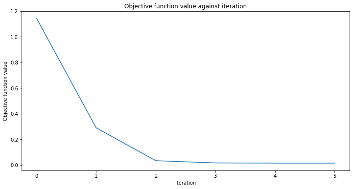
optimizer=L_BFGS_B(maxiter=5),
callback=callback_graph,
)
[30]:
# create empty array for callback to store evaluations of the objective function
objective_func_vals = []
plt.rcParams["figure.figsize"] = (12, 6)

# fit to data
regressor.fit(X, y)

# return to default figsize
plt.rcParams["figure.figsize"] = (6, 4)

# score the result
regressor.score(X, y)
[30]:
0.9769994291935522
[31]:
# plot target function
plt.plot(X_, f(X_), "r--")

# plot data
plt.plot(X, y, "bo")

# plot fitted line
y_ = regressor.predict(X_)
plt.plot(X_, y_, "g-")
plt.show()
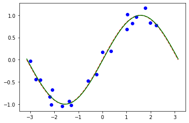
Similarly to the classification models, we can obtain an array of trained weights by querying a corresponding property of the model. In this model we have only one parameter defined as param_y above.
[32]:
regressor.weights
[32]:
array([-1.58870599])
Variational Quantum Regressor (VQR) 를 이용한 회귀#
Similar to the VQC for classification, the VQR is a special variant of the NeuralNetworkRegressor with a EstimatorQNN. By default it considers the L2Loss function to minimize the mean squared error between predictions and targets.
[33]:
vqr = VQR(
feature_map=feature_map,
ansatz=ansatz,
optimizer=L_BFGS_B(maxiter=5),
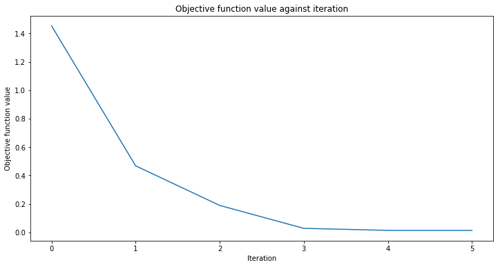
callback=callback_graph,
)
[34]:
# create empty array for callback to store evaluations of the objective function
objective_func_vals = []
plt.rcParams["figure.figsize"] = (12, 6)

# fit regressor
vqr.fit(X, y)

# return to default figsize
plt.rcParams["figure.figsize"] = (6, 4)

# score result
vqr.score(X, y)
[34]:
0.9769955693935385
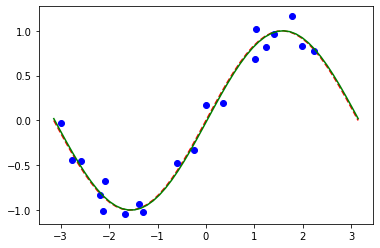
[35]:
# plot target function
plt.plot(X_, f(X_), "r--")

# plot data
plt.plot(X, y, "bo")

# plot fitted line
y_ = vqr.predict(X_)
plt.plot(X_, y_, "g-")
plt.show()
[36]:
import qiskit.tools.jupyter

%qiskit_version_table
%qiskit_copyright
Version Information
| Qiskit Software | Version |
|---|---|
qiskit-terra | 0.24.0 |
qiskit-aer | 0.12.0 |
qiskit-ignis | 0.6.0 |
qiskit-ibmq-provider | 0.20.2 |
qiskit | 0.43.0 |
qiskit-machine-learning | 0.7.0 |
| System information | |
| Python version | 3.8.8 |
| Python compiler | Clang 10.0.0 |
| Python build | default, Apr 13 2021 12:59:45 |
| OS | Darwin |
| CPUs | 8 |
| Memory (Gb) | 32.0 |
| Tue Jun 13 16:39:30 2023 CEST | |
This code is a part of Qiskit
© Copyright IBM 2017, 2023.
This code is licensed under the Apache License, Version 2.0. You may
obtain a copy of this license in the LICENSE.txt file in the root directory
of this source tree or at http://www.apache.org/licenses/LICENSE-2.0.
Any modifications or derivative works of this code must retain this
copyright notice, and modified files need to carry a notice indicating
that they have been altered from the originals.