Note
This page was generated from docs/tutorials/05_torch_connector.ipynb.
Torch Connector and Hybrid QNNs
This tutorial introduces the TorchConnector class, and demonstrates how it allows for a natural integration of any NeuralNetwork from Qiskit Machine Learning into a PyTorch workflow. TorchConnector takes a NeuralNetwork and makes it available as a PyTorch Module. The resulting module can be seamlessly incorporated into PyTorch classical architectures and trained jointly without additional considerations, enabling the development and testing of novel hybrid
quantum-classical machine learning architectures.
Content:
Part 1: Simple Classification & Regression
The first part of this tutorial shows how quantum neural networks can be trained using PyTorch’s automatic differentiation engine (torch.autograd, link) for simple classification and regression tasks.
-
Classification with PyTorch and
EstimatorQNNClassification with PyTorch and
SamplerQNN
-
Regression with PyTorch and
EstimatorQNN
Part 2: MNIST Classification, Hybrid QNNs
The second part of this tutorial illustrates how to embed a (Quantum) NeuralNetwork into a target PyTorch workflow (in this case, a typical CNN architecture) to classify MNIST data in a hybrid quantum-classical manner.
[1]:
# Necessary imports

import numpy as np
import matplotlib.pyplot as plt

from torch import Tensor
from torch.nn import Linear, CrossEntropyLoss, MSELoss
from torch.optim import LBFGS

from qiskit import QuantumCircuit
from qiskit.circuit import Parameter
from qiskit.circuit.library import RealAmplitudes, ZZFeatureMap
from qiskit_machine_learning.utils import algorithm_globals
from qiskit_machine_learning.neural_networks import SamplerQNN, EstimatorQNN
from qiskit_machine_learning.connectors import TorchConnector

# Set seed for random generators
algorithm_globals.random_seed = 42
Part 1: Simple Classification & Regression
1. Classification
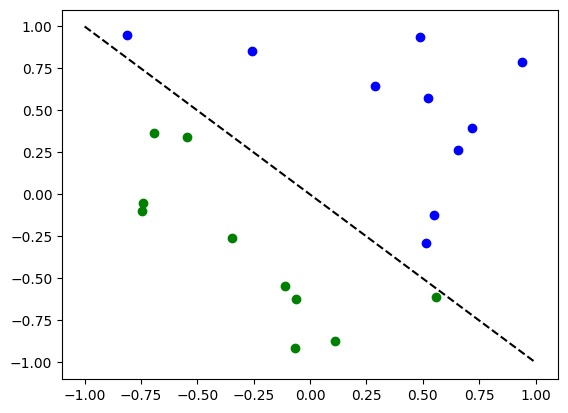
First, we show how TorchConnector allows to train a Quantum NeuralNetwork to solve a classification tasks using PyTorch’s automatic differentiation engine. In order to illustrate this, we will perform binary classification on a randomly generated dataset.
[2]:
# Generate random dataset

# Select dataset dimension (num_inputs) and size (num_samples)
num_inputs = 2
num_samples = 20

# Generate random input coordinates (X) and binary labels (y)
X = 2 * algorithm_globals.random.random([num_samples, num_inputs]) - 1
y01 = 1 * (np.sum(X, axis=1) >= 0)  # in { 0,  1}, y01 will be used for SamplerQNN example
y = 2 * y01 - 1  # in {-1, +1}, y will be used for EstimatorQNN example

# Convert to torch Tensors
X_ = Tensor(X)
y01_ = Tensor(y01).reshape(len(y)).long()
y_ = Tensor(y).reshape(len(y), 1)

# Plot dataset
for x, y_target in zip(X, y):
    if y_target == 1:
        plt.plot(x[0], x[1], "bo")
    else:
        plt.plot(x[0], x[1], "go")
plt.plot([-1, 1], [1, -1], "--", color="black")
plt.show()
A. Classification with PyTorch and EstimatorQNN
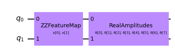
Linking an EstimatorQNN to PyTorch is relatively straightforward. Here we illustrate this by using the EstimatorQNN constructed from a feature map and an ansatz.
[3]:
# Set up a circuit
feature_map = ZZFeatureMap(num_inputs)
ansatz = RealAmplitudes(num_inputs)
qc = QuantumCircuit(num_inputs)
qc.compose(feature_map, inplace=True)
qc.compose(ansatz, inplace=True)
qc.draw(output="mpl", style="clifford")
[3]:
[4]:
from qiskit.primitives import StatevectorEstimator as Estimator

estimator = Estimator()
# Setup QNN
qnn1 = EstimatorQNN(
    circuit=qc,
    input_params=feature_map.parameters,
    weight_params=ansatz.parameters,
    estimator=estimator,
)

# Set up PyTorch module
# Note: If we don't explicitly declare the initial weights
# they are chosen uniformly at random from [-1, 1].
initial_weights = 0.1 * (2 * algorithm_globals.random.random(qnn1.num_weights) - 1)
model1 = TorchConnector(qnn1, initial_weights=initial_weights)
print("Initial weights: ", initial_weights)
No gradient function provided, creating a gradient function. If your Estimator requires transpilation, please provide a pass manager.
Initial weights:  [-0.01256962  0.06653564  0.04005302 -0.03752667  0.06645196  0.06095287
 -0.02250432 -0.04233438]
[5]:
# Test with a single input
model1(X_[0, :])
[5]:
tensor([-0.3230], grad_fn=<_TorchNNFunctionBackward>)
Optimizer
The choice of optimizer for training any machine learning model can be crucial in determining the success of our training’s outcome. When using TorchConnector, we get access to all of the optimizer algorithms defined in the [torch.optim] package (link). Some of the most famous algorithms used in popular machine learning architectures include Adam, SGD, or Adagrad. However, for this tutorial we will be using the L-BFGS algorithm
(torch.optim.LBFGS), one of the most well know second-order optimization algorithms for numerical optimization.
Loss Function
As for the loss function, we can also take advantage of PyTorch’s pre-defined modules from torch.nn, such as the Cross-Entropy or Mean Squared Error losses.
💡 Clarification : In classical machine learning, the general rule of thumb is to apply a Cross-Entropy loss to classification tasks, and MSE loss to regression tasks. However, this recommendation is given under the assumption that the output of the classification network is a class probability value in the EstimatorQNN does not include such layer, and we don’t apply any mapping to
the output (the following section shows an example of application of parity mapping with SamplerQNNs), the QNN’s output can take any value in the range
[6]:
# Define optimizer and loss
optimizer = LBFGS(model1.parameters())
f_loss = MSELoss(reduction="sum")

# Start training
model1.train()  # set model to training mode


# Note from (https://pytorch.org/docs/stable/optim.html):
# Some optimization algorithms such as LBFGS need to
# reevaluate the function multiple times, so you have to
# pass in a closure that allows them to recompute your model.
# The closure should clear the gradients, compute the loss,
# and return it.
def closure():
    optimizer.zero_grad()  # Initialize/clear gradients
    loss = f_loss(model1(X_), y_)  # Evaluate loss function
    loss.backward()  # Backward pass
    print(loss.item())  # Print loss
    return loss


# Run optimizer step4
optimizer.step(closure)
25.5554141998291
22.84799575805664
19.960691452026367
19.278564453125
19.302776336669922
18.135221481323242
17.3953857421875
21.259014129638672
25.036849975585938
21.41744041442871
27.72951889038086
23.96538543701172
25.911020278930664
25.522098541259766
24.56904411315918
20.529380798339844
24.416887283325195
21.865007400512695
25.827163696289062
26.854175567626953
[6]:
tensor(25.5554, grad_fn=<MseLossBackward0>)
[7]:
# Evaluate model and compute accuracy
model1.eval()
y_predict = []
for x, y_target in zip(X, y):
    output = model1(Tensor(x))
    y_predict += [np.sign(output.detach().numpy())[0]]

print("Accuracy:", sum(y_predict == y) / len(y))

# Plot results
# red == wrongly classified
for x, y_target, y_p in zip(X, y, y_predict):
    if y_target == 1:
        plt.plot(x[0], x[1], "bo")
    else:
        plt.plot(x[0], x[1], "go")
    if y_target != y_p:
        plt.scatter(x[0], x[1], s=200, facecolors="none", edgecolors="r", linewidths=2)
plt.plot([-1, 1], [1, -1], "--", color="black")
plt.show()
Accuracy: 0.65
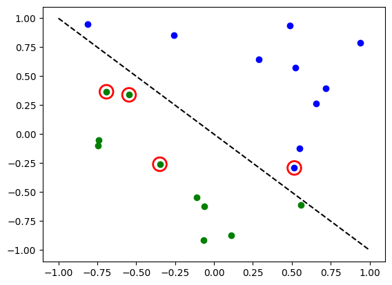
The red circles indicate wrongly classified data points.
B. Classification with PyTorch and SamplerQNN
Linking a SamplerQNN to PyTorch requires a bit more attention than EstimatorQNN. Without the correct setup, backpropagation is not possible.
In particular, we must make sure that we are returning a dense array of probabilities in the network’s forward pass (sparse=False). This parameter is set up to False by default, so we just have to make sure that it has not been changed.
⚠️ Attention: If we define a custom interpret function ( in the example: parity), we must remember to explicitly provide the desired output shape ( in the example: 2). For more info on the initial parameter setup for SamplerQNN, please check out the official qiskit documentation.
[8]:
# Define feature map and ansatz
feature_map = ZZFeatureMap(num_inputs)
ansatz = RealAmplitudes(num_inputs, entanglement="linear", reps=1)

# Define quantum circuit of num_qubits = input dim
# Append feature map and ansatz
qc = QuantumCircuit(num_inputs)
qc.compose(feature_map, inplace=True)
qc.compose(ansatz, inplace=True)

from qiskit.primitives import StatevectorSampler as Sampler

sampler = Sampler()

# Define SamplerQNN and initial setup
parity = lambda x: "{:b}".format(x).count("1") % 2  # optional interpret function
output_shape = 2  # parity = 0, 1
qnn2 = SamplerQNN(
    circuit=qc,
    input_params=feature_map.parameters,
    weight_params=ansatz.parameters,
    interpret=parity,
    output_shape=output_shape,
    sampler=sampler,
)

# Set up PyTorch module
# Reminder: If we don't explicitly declare the initial weights
# they are chosen uniformly at random from [-1, 1].
initial_weights = 0.1 * (2 * algorithm_globals.random.random(qnn2.num_weights) - 1)
print("Initial weights: ", initial_weights)
model2 = TorchConnector(qnn2, initial_weights)
No gradient function provided, creating a gradient function. If your Sampler requires transpilation, please provide a pass manager.
Initial weights: [ 0.0364991 -0.0720495 -0.06001836 -0.09852755]
For a reminder on optimizer and loss function choices, you can go back to this section.
[9]:
# Define model, optimizer, and loss
optimizer = LBFGS(model2.parameters())
f_loss = CrossEntropyLoss()  # Our output will be in the [0,1] range

# Start training
model2.train()


# Define LBFGS closure method (explained in previous section)
def closure():
    optimizer.zero_grad(set_to_none=True)  # Initialize gradient
    loss = f_loss(model2(X_), y01_)  # Calculate loss
    loss.backward()  # Backward pass

    print(loss.item())  # Print loss
    return loss


# Run optimizer (LBFGS requires closure)
optimizer.step(closure);
0.6882659196853638
0.6913522481918335
0.691373348236084
0.6647081971168518
0.6528792381286621
0.6443885564804077
0.6994273066520691
0.7723010182380676
0.7129653096199036
0.6990549564361572
0.6716065406799316
0.7544995546340942
0.6825253367424011
0.6849457621574402
0.7210066914558411
0.7053173184394836
0.6781826019287109
0.7493025064468384
0.7046105265617371
0.6678831577301025
[10]:
# Evaluate model and compute accuracy
model2.eval()
y_predict = []
for x in X:
    output = model2(Tensor(x))
    y_predict += [np.argmax(output.detach().numpy())]

print("Accuracy:", sum(y_predict == y01) / len(y01))

# plot results
# red == wrongly classified
for x, y_target, y_ in zip(X, y01, y_predict):
    if y_target == 1:
        plt.plot(x[0], x[1], "bo")
    else:
        plt.plot(x[0], x[1], "go")
    if y_target != y_:
        plt.scatter(x[0], x[1], s=200, facecolors="none", edgecolors="r", linewidths=2)
plt.plot([-1, 1], [1, -1], "--", color="black")
plt.show()
Accuracy: 0.65

The red circles indicate wrongly classified data points.
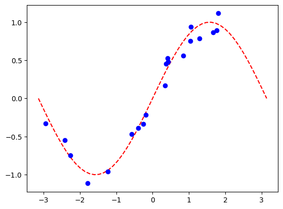
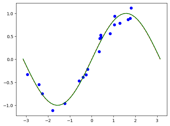
2. Regression
We use a model based on the EstimatorQNN to also illustrate how to perform a regression task. The chosen dataset in this case is randomly generated following a sine wave.
[11]:
# Generate random dataset

num_samples = 20
eps = 0.2
lb, ub = -np.pi, np.pi
f = lambda x: np.sin(x)

X = (ub - lb) * algorithm_globals.random.random([num_samples, 1]) + lb
y = f(X) + eps * (2 * algorithm_globals.random.random([num_samples, 1]) - 1)
plt.plot(np.linspace(lb, ub), f(np.linspace(lb, ub)), "r--")
plt.plot(X, y, "bo")
plt.show()
A. Regression with PyTorch and EstimatorQNN
The network definition and training loop will be analogous to those of the classification task using EstimatorQNN. In this case, we define our own feature map and ansatz, but let’s do it a little different.
[12]:
# Construct simple feature map
param_x = Parameter("x")
feature_map = QuantumCircuit(1, name="fm")
feature_map.ry(param_x, 0)

# Construct simple parameterized ansatz
param_y = Parameter("y")
ansatz = QuantumCircuit(1, name="vf")
ansatz.ry(param_y, 0)

qc = QuantumCircuit(1)
qc.compose(feature_map, inplace=True)
qc.compose(ansatz, inplace=True)

# Construct QNN
qnn3 = EstimatorQNN(
    circuit=qc, input_params=[param_x], weight_params=[param_y], estimator=estimator
)

# Set up PyTorch module
# Reminder: If we don't explicitly declare the initial weights
# they are chosen uniformly at random from [-1, 1].
initial_weights = 0.1 * (2 * algorithm_globals.random.random(qnn3.num_weights) - 1)
model3 = TorchConnector(qnn3, initial_weights)
No gradient function provided, creating a gradient function. If your Estimator requires transpilation, please provide a pass manager.
For a reminder on optimizer and loss function choices, you can go back to this section.
[13]:
# Define optimizer and loss function
optimizer = LBFGS(model3.parameters())
f_loss = MSELoss(reduction="sum")

# Start training
model3.train()  # set model to training mode


# Define objective function
def closure():
    optimizer.zero_grad(set_to_none=True)  # Initialize gradient
    loss = f_loss(model3(Tensor(X)), Tensor(y))  # Compute batch loss
    loss.backward()  # Backward pass
    print(loss.item())  # Print loss
    return loss


# Run optimizer
optimizer.step(closure)
14.9714994430542
2.9661648273468018
8.842530250549316
0.4107576608657837
0.2440420687198639
0.25234255194664
0.2235121876001358
0.27348196506500244
0.2771543860435486
0.25521329045295715
0.2350853979587555
0.24883446097373962
0.2356414496898651
0.24924549460411072
0.2499208003282547
0.2549074590206146
0.2685125470161438
0.24676817655563354
0.23014217615127563
0.27330708503723145
[13]:
tensor(14.9715, grad_fn=<MseLossBackward0>)
[14]:
# Plot target function
plt.plot(np.linspace(lb, ub), f(np.linspace(lb, ub)), "r--")

# Plot data
plt.plot(X, y, "bo")

# Plot fitted line
model3.eval()
y_ = []
for x in np.linspace(lb, ub):
    output = model3(Tensor([x]))
    y_ += [output.detach().numpy()[0]]
plt.plot(np.linspace(lb, ub), y_, "g-")
plt.show()
Part 2: MNIST Classification, Hybrid QNNs
In this second part, we show how to leverage a hybrid quantum-classical neural network using TorchConnector, to perform a more complex image classification task on the MNIST handwritten digits dataset.
For a more detailed (pre-TorchConnector) explanation on hybrid quantum-classical neural networks, you can check out the corresponding section in the Qiskit Textbook repository.
[15]:
# Additional torch-related imports
import torch
from torch import cat, no_grad, manual_seed
from torch.utils.data import DataLoader
from torchvision import datasets, transforms
import torch.optim as optim
from torch.nn import (
    Module,
    Conv2d,
    Linear,
    Dropout2d,
    NLLLoss,
    MaxPool2d,
    Flatten,
    Sequential,
    ReLU,
)
import torch.nn.functional as F
Step 1: Defining Data-loaders for train and test
We take advantage of the torchvision API to directly load a subset of the MNIST dataset and define torch DataLoaders (link) for train and test.
[16]:
# Train Dataset
# -------------

# Set train shuffle seed (for reproducibility)
manual_seed(42)

batch_size = 1
n_samples = 100  # We will concentrate on the first 100 samples

# Use pre-defined torchvision function to load MNIST train data
X_train = datasets.MNIST(
    root="./data", train=True, download=True, transform=transforms.Compose([transforms.ToTensor()])
)

# Filter out labels (originally 0-9), leaving only labels 0 and 1
idx = np.append(
    np.where(X_train.targets == 0)[0][:n_samples], np.where(X_train.targets == 1)[0][:n_samples]
)
X_train.data = X_train.data[idx]
X_train.targets = X_train.targets[idx]

# Define torch dataloader with filtered data
train_loader = DataLoader(X_train, batch_size=batch_size, shuffle=True)
Downloading http://yann.lecun.com/exdb/mnist/train-images-idx3-ubyte.gz
Failed to download (trying next):
HTTP Error 403: Forbidden

Downloading https://ossci-datasets.s3.amazonaws.com/mnist/train-images-idx3-ubyte.gz
Downloading https://ossci-datasets.s3.amazonaws.com/mnist/train-images-idx3-ubyte.gz to ./data/MNIST/raw/train-images-idx3-ubyte.gz
100.0%
Extracting ./data/MNIST/raw/train-images-idx3-ubyte.gz to ./data/MNIST/raw

Downloading http://yann.lecun.com/exdb/mnist/train-labels-idx1-ubyte.gz
Failed to download (trying next):
HTTP Error 403: Forbidden

Downloading https://ossci-datasets.s3.amazonaws.com/mnist/train-labels-idx1-ubyte.gz
Downloading https://ossci-datasets.s3.amazonaws.com/mnist/train-labels-idx1-ubyte.gz to ./data/MNIST/raw/train-labels-idx1-ubyte.gz
100.0%
Extracting ./data/MNIST/raw/train-labels-idx1-ubyte.gz to ./data/MNIST/raw

Downloading http://yann.lecun.com/exdb/mnist/t10k-images-idx3-ubyte.gz
Failed to download (trying next):
HTTP Error 403: Forbidden

Downloading https://ossci-datasets.s3.amazonaws.com/mnist/t10k-images-idx3-ubyte.gz
Downloading https://ossci-datasets.s3.amazonaws.com/mnist/t10k-images-idx3-ubyte.gz to ./data/MNIST/raw/t10k-images-idx3-ubyte.gz
100.0%
Extracting ./data/MNIST/raw/t10k-images-idx3-ubyte.gz to ./data/MNIST/raw

Downloading http://yann.lecun.com/exdb/mnist/t10k-labels-idx1-ubyte.gz
Failed to download (trying next):
HTTP Error 403: Forbidden

Downloading https://ossci-datasets.s3.amazonaws.com/mnist/t10k-labels-idx1-ubyte.gz
Downloading https://ossci-datasets.s3.amazonaws.com/mnist/t10k-labels-idx1-ubyte.gz to ./data/MNIST/raw/t10k-labels-idx1-ubyte.gz
100.0%
Extracting ./data/MNIST/raw/t10k-labels-idx1-ubyte.gz to ./data/MNIST/raw
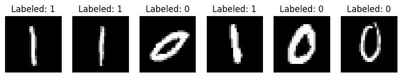
If we perform a quick visualization we can see that the train dataset consists of images of handwritten 0s and 1s.
[17]:
n_samples_show = 6

data_iter = iter(train_loader)
fig, axes = plt.subplots(nrows=1, ncols=n_samples_show, figsize=(10, 3))

while n_samples_show > 0:
    images, targets = data_iter.__next__()

    axes[n_samples_show - 1].imshow(images[0, 0].numpy().squeeze(), cmap="gray")
    axes[n_samples_show - 1].set_xticks([])
    axes[n_samples_show - 1].set_yticks([])
    axes[n_samples_show - 1].set_title("Labeled: {}".format(targets[0].item()))

    n_samples_show -= 1
[18]:
# Test Dataset
# -------------

# Set test shuffle seed (for reproducibility)
# manual_seed(5)

n_samples = 50

# Use pre-defined torchvision function to load MNIST test data
X_test = datasets.MNIST(
    root="./data", train=False, download=True, transform=transforms.Compose([transforms.ToTensor()])
)

# Filter out labels (originally 0-9), leaving only labels 0 and 1
idx = np.append(
    np.where(X_test.targets == 0)[0][:n_samples], np.where(X_test.targets == 1)[0][:n_samples]
)
X_test.data = X_test.data[idx]
X_test.targets = X_test.targets[idx]

# Define torch dataloader with filtered data
test_loader = DataLoader(X_test, batch_size=batch_size, shuffle=True)
Step 2: Defining the QNN and Hybrid Model
This second step shows the power of the TorchConnector. After defining our quantum neural network layer (in this case, a EstimatorQNN), we can embed it into a layer in our torch Module by initializing a torch connector as TorchConnector(qnn).
⚠️ Attention: In order to have an adequate gradient backpropagation in hybrid models, we MUST set the initial parameter input_gradients to TRUE during the qnn initialization.
[19]:
# Define and create QNN
def create_qnn():
    feature_map = ZZFeatureMap(2)
    ansatz = RealAmplitudes(2, reps=1)
    qc = QuantumCircuit(2)
    qc.compose(feature_map, inplace=True)
    qc.compose(ansatz, inplace=True)

    # REMEMBER TO SET input_gradients=True FOR ENABLING HYBRID GRADIENT BACKPROP
    qnn = EstimatorQNN(
        circuit=qc,
        input_params=feature_map.parameters,
        weight_params=ansatz.parameters,
        input_gradients=True,
        estimator=estimator,
    )
    return qnn


qnn4 = create_qnn()
No gradient function provided, creating a gradient function. If your Estimator requires transpilation, please provide a pass manager.
[20]:
# Define torch NN module


class Net(Module):
    def __init__(self, qnn):
        super().__init__()
        self.conv1 = Conv2d(1, 2, kernel_size=5)
        self.conv2 = Conv2d(2, 16, kernel_size=5)
        self.dropout = Dropout2d()
        self.fc1 = Linear(256, 64)
        self.fc2 = Linear(64, 2)  # 2-dimensional input to QNN
        self.qnn = TorchConnector(qnn)  # Apply torch connector, weights chosen
        # uniformly at random from interval [-1,1].
        self.fc3 = Linear(1, 1)  # 1-dimensional output from QNN

    def forward(self, x):
        x = F.relu(self.conv1(x))
        x = F.max_pool2d(x, 2)
        x = F.relu(self.conv2(x))
        x = F.max_pool2d(x, 2)
        x = self.dropout(x)
        x = x.view(x.shape[0], -1)
        x = F.relu(self.fc1(x))
        x = self.fc2(x)
        x = self.qnn(x)  # apply QNN
        x = self.fc3(x)
        return cat((x, 1 - x), -1)


model4 = Net(qnn4)
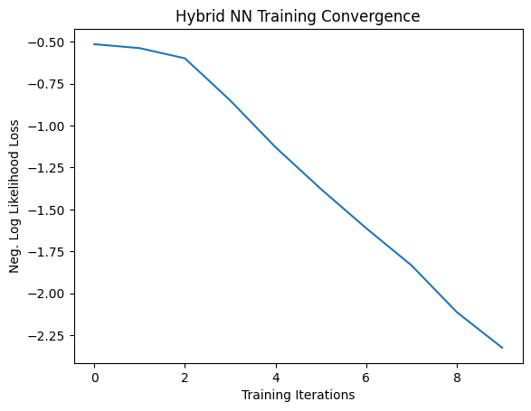
Step 3: Training
[21]:
# Define model, optimizer, and loss function
optimizer = optim.Adam(model4.parameters(), lr=0.001)
loss_func = NLLLoss()

# Start training
epochs = 10  # Set number of epochs
loss_list = []  # Store loss history
model4.train()  # Set model to training mode

for epoch in range(epochs):
    total_loss = []
    for batch_idx, (data, target) in enumerate(train_loader):
        optimizer.zero_grad(set_to_none=True)  # Initialize gradient
        output = model4(data)  # Forward pass
        loss = loss_func(output, target)  # Calculate loss
        loss.backward()  # Backward pass
        optimizer.step()  # Optimize weights
        total_loss.append(loss.item())  # Store loss
    loss_list.append(sum(total_loss) / len(total_loss))
    print("Training [{:.0f}%]\tLoss: {:.4f}".format(100.0 * (epoch + 1) / epochs, loss_list[-1]))
Training [10%]  Loss: -1.1616
Training [20%]  Loss: -1.5284
Training [30%]  Loss: -1.7868
Training [40%]  Loss: -1.9830
Training [50%]  Loss: -2.2307
Training [60%]  Loss: -2.4558
Training [70%]  Loss: -2.6722
Training [80%]  Loss: -2.8756
Training [90%]  Loss: -3.1111
Training [100%] Loss: -3.3085
[22]:
# Plot loss convergence
plt.plot(loss_list)
plt.title("Hybrid NN Training Convergence")
plt.xlabel("Training Iterations")
plt.ylabel("Neg. Log Likelihood Loss")
plt.show()
Now we’ll save the trained model, just to show how a hybrid model can be saved and re-used later for inference. To save and load hybrid models, when using the TorchConnector, follow the PyTorch recommendations of saving and loading the models.
[23]:
torch.save(model4.state_dict(), "model4.pt")
Step 4: Evaluation
We start from recreating the model and loading the state from the previously saved file. You create a QNN layer using another simulator or a real hardware. So, you can train a model on real hardware available on the cloud and then for inference use a simulator or vice verse. For a sake of simplicity we create a new quantum neural network in the same way as above.
[24]:
qnn5 = create_qnn()
model5 = Net(qnn5)
model5.load_state_dict(torch.load("model4.pt"))
No gradient function provided, creating a gradient function. If your Estimator requires transpilation, please provide a pass manager.
/tmp/ipykernel_4510/2057927024.py:3: FutureWarning: You are using `torch.load` with `weights_only=False` (the current default value), which uses the default pickle module implicitly. It is possible to construct malicious pickle data which will execute arbitrary code during unpickling (See https://github.com/pytorch/pytorch/blob/main/SECURITY.md#untrusted-models for more details). In a future release, the default value for `weights_only` will be flipped to `True`. This limits the functions that could be executed during unpickling. Arbitrary objects will no longer be allowed to be loaded via this mode unless they are explicitly allowlisted by the user via `torch.serialization.add_safe_globals`. We recommend you start setting `weights_only=True` for any use case where you don't have full control of the loaded file. Please open an issue on GitHub for any issues related to this experimental feature.
  model5.load_state_dict(torch.load("model4.pt"))
[24]:
<All keys matched successfully>
[25]:
model5.eval()  # set model to evaluation mode
with no_grad():

    correct = 0
    for batch_idx, (data, target) in enumerate(test_loader):
        output = model5(data)
        if len(output.shape) == 1:
            output = output.reshape(1, *output.shape)

        pred = output.argmax(dim=1, keepdim=True)
        correct += pred.eq(target.view_as(pred)).sum().item()

        loss = loss_func(output, target)
        total_loss.append(loss.item())

    print(
        "Performance on test data:\n\tLoss: {:.4f}\n\tAccuracy: {:.1f}%".format(
            sum(total_loss) / len(total_loss), correct / len(test_loader) / batch_size * 100
        )
    )
Performance on test data:
        Loss: -3.3448
        Accuracy: 100.0%
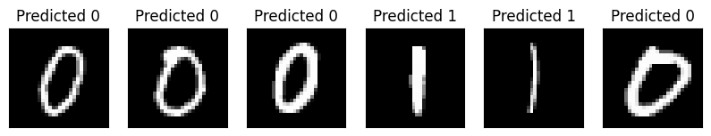
[26]:
# Plot predicted labels

n_samples_show = 6
count = 0
fig, axes = plt.subplots(nrows=1, ncols=n_samples_show, figsize=(10, 3))

model5.eval()
with no_grad():
    for batch_idx, (data, target) in enumerate(test_loader):
        if count == n_samples_show:
            break
        output = model5(data[0:1])
        if len(output.shape) == 1:
            output = output.reshape(1, *output.shape)

        pred = output.argmax(dim=1, keepdim=True)

        axes[count].imshow(data[0].numpy().squeeze(), cmap="gray")

        axes[count].set_xticks([])
        axes[count].set_yticks([])
        axes[count].set_title("Predicted {}".format(pred.item()))

        count += 1
🎉🎉🎉🎉 You are now able to experiment with your own hybrid datasets and architectures using Qiskit Machine Learning. Good Luck!
[27]:
import tutorial_magics

%qiskit_version_table
%qiskit_copyright
Version Information
| Software | Version |
|---|---|
qiskit | 1.3.1 |
qiskit_machine_learning | 0.8.2 |
| System information | |
| Python version | 3.10.15 |
| OS | Linux |
| Fri Dec 20 15:48:50 2024 UTC | |
This code is a part of a Qiskit project
© Copyright IBM 2017, 2024.
This code is licensed under the Apache License, Version 2.0. You may
obtain a copy of this license in the LICENSE.txt file in the root directory
of this source tree or at http://www.apache.org/licenses/LICENSE-2.0.
Any modifications or derivative works of this code must retain this
copyright notice, and modified files need to carry a notice indicating
that they have been altered from the originals.