참고
이 페이지는 `docs/tutorials/07_pegasos_qsvc.ipynb`에서 생성되었다.
Pegasos Quantum Support Vector Classifier#
There’s another SVM based algorithm that benefits from the quantum kernel method. Here, we introduce an implementation of a another classification algorithm, which is an alternative version to the QSVC available in Qiskit Machine Learning and shown in the “Quantum Kernel Machine Learning” tutorial. This classification algorithm implements the Pegasos algorithm from the paper “Pegasos: Primal Estimated sub-GrAdient SOlver for SVM” by Shalev-Shwartz et al., see:
https://home.ttic.edu/~nati/Publications/PegasosMPB.pdf.
이 알고리즘은 scikit-learn 패키지에 있는 dual optimization의 대안이고, 커널 트릭의 이점을 가지며 학습 복잡도가 학습 세트의 크기와 무관하다. 따라서 PegasosQSVC 는 방대한 크기의 학습 세트에 대해 QSVC보다 빠르게 학습할 수 있을 것이다.
이 알고리즘은 일부 하이퍼 파라미터로 ``QSVC``를 직접 대체하는데 사용될 수 있다.
Let’s generate some data:
[1]:
from sklearn.datasets import make_blobs

# example dataset
features, labels = make_blobs(n_samples=20, n_features=2, centers=2, random_state=3, shuffle=True)
회전 인코딩과 호환성을 보장하기 위해 데이터를 전처리하고 이를 학습 및 테스트 데이터 세트로 분할한다.
[2]:
import numpy as np

from sklearn.model_selection import train_test_split
from sklearn.preprocessing import MinMaxScaler

features = MinMaxScaler(feature_range=(0, np.pi)).fit_transform(features)

train_features, test_features, train_labels, test_labels = train_test_split(
    features, labels, train_size=15, shuffle=False
)
데이터 세트에는 두 가지 특징이 있으므로 데이터 세트의 특징 수에 따라 큐비트를 설정한다.
그리고 나서 \(tau`를 학습 과정에서 수행되는 단계 수로 설정한다. 알고리즘에는 조기 종료 기준이 없다. 알고리즘은 모든 :math:`tau\) 단계를 반복한다.
그리고 마지막은 하이퍼 파라미터 :math:`C`이다. 이것은 양의 정규화 매개변수다. 정규화의 강도는 :math:`C`에 반비례한다. 더 작은 :math:`C`는 일반적으로 과적합을 방지하는데 도움이 되는 작은 가중치를 유도한다. 그러나 이 알고리즘의 특성으로 인해 일부 계산 단계는 큰 :math:`C`이 된다. 그러므로 :math:`C`가 클수록 알고리즘의 성능이 크게 향상된다. 만약 데이터가 feature space에서 선형으로 분리할 수 있으면 :math:`C`를 큰 값으로 선택해야 한다. 그렇지 않다면, 과적합을 방지하기 위해 :math:`C`를 더 작게 선택해야 한다.
[3]:
# number of qubits is equal to the number of features
num_qubits = 2

# number of steps performed during the training procedure
tau = 100

# regularization parameter
C = 1000
알고리즘은 다음을 사용하여 실행된다:
The default fidelity instantiated in
FidelityQuantumKernelZFeatureMap에서 생성된 양자 커널
[4]:
from qiskit import BasicAer
from qiskit.circuit.library import ZFeatureMap
from qiskit_algorithms.utils import algorithm_globals

from qiskit_machine_learning.kernels import FidelityQuantumKernel

algorithm_globals.random_seed = 12345

feature_map = ZFeatureMap(feature_dimension=num_qubits, reps=1)

qkernel = FidelityQuantumKernel(feature_map=feature_map)
PegasosQSVC 구현은 scikit-learn 인터페이스와 호환되며 매우 표준적인 모델 훈련 방식을 가지고 있다. 생성자에서 알고리즘의 매개변수를 전달하는데, 이 경우 정규화 하이퍼-파라미터 \(C\) 와 여러 단계가 있다.
그런 다음 모델을 훈련하고 적합한 분류기를 반환하는 fit 메서드에 훈련 데이터의 특징과 레이블을 전달한다.
그런 다음 테스트 데이터의 특징과 레이블을 사용하여 모델에 점수를 매긴다.
[5]:
from qiskit_machine_learning.algorithms import PegasosQSVC

pegasos_qsvc = PegasosQSVC(quantum_kernel=qkernel, C=C, num_steps=tau)

# training
pegasos_qsvc.fit(train_features, train_labels)

# testing
pegasos_score = pegasos_qsvc.score(test_features, test_labels)
print(f"PegasosQSVC classification test score: {pegasos_score}")
PegasosQSVC classification test score: 1.0
시각화를 위해 MinMaxScaler에 적용한 최소값과 최대값을 포괄하는 사전 정의된 단계의 격자점을 만든다. 또한 훈련 및 테스트 샘플의 더 나은 표현을 위해 격자에 약간의 마진(margin)을 추가한다.
[6]:
grid_step = 0.2
margin = 0.2
grid_x, grid_y = np.meshgrid(
    np.arange(-margin, np.pi + margin, grid_step), np.arange(-margin, np.pi + margin, grid_step)
)
격자를 모델과 호환되는 모양으로 변환하며 모양은 (n_samples, n_features) 이어야 한다. 그런 다음 각 격자점에 대해 레이블을 예측한다. 예측된 레이블은 격자점의 색상을 지정하는데 사용된다.
[7]:
meshgrid_features = np.column_stack((grid_x.ravel(), grid_y.ravel()))
meshgrid_colors = pegasos_qsvc.predict(meshgrid_features)
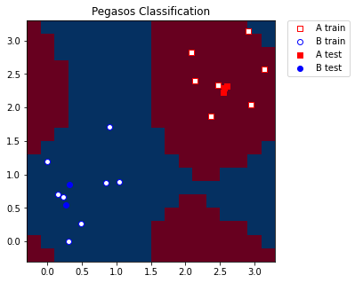
마지막으로 모델에서 얻은 레이블/색상에 따라 격자를 그린다. 훈련 및 테스트 샘플들도 그림에 표시한다.
[8]:
import matplotlib.pyplot as plt

plt.figure(figsize=(5, 5))
meshgrid_colors = meshgrid_colors.reshape(grid_x.shape)
plt.pcolormesh(grid_x, grid_y, meshgrid_colors, cmap="RdBu", shading="auto")

plt.scatter(
    train_features[:, 0][train_labels == 0],
    train_features[:, 1][train_labels == 0],
    marker="s",
    facecolors="w",
    edgecolors="r",
    label="A train",
)
plt.scatter(
    train_features[:, 0][train_labels == 1],
    train_features[:, 1][train_labels == 1],
    marker="o",
    facecolors="w",
    edgecolors="b",
    label="B train",
)

plt.scatter(
    test_features[:, 0][test_labels == 0],
    test_features[:, 1][test_labels == 0],
    marker="s",
    facecolors="r",
    edgecolors="r",
    label="A test",
)
plt.scatter(
    test_features[:, 0][test_labels == 1],
    test_features[:, 1][test_labels == 1],
    marker="o",
    facecolors="b",
    edgecolors="b",
    label="B test",
)

plt.legend(bbox_to_anchor=(1.05, 1), loc="upper left", borderaxespad=0.0)
plt.title("Pegasos Classification")
plt.show()
[9]:
import qiskit.tools.jupyter

%qiskit_version_table
%qiskit_copyright
Version Information
| Qiskit Software | Version |
|---|---|
qiskit-terra | 0.22.0 |
qiskit-aer | 0.11.0 |
qiskit-ignis | 0.7.0 |
qiskit | 0.33.0 |
qiskit-machine-learning | 0.5.0 |
| System information | |
| Python version | 3.7.9 |
| Python compiler | MSC v.1916 64 bit (AMD64) |
| Python build | default, Aug 31 2020 17:10:11 |
| OS | Windows |
| CPUs | 4 |
| Memory (Gb) | 31.837730407714844 |
| Thu Oct 13 10:42:49 2022 GMT Daylight Time | |
This code is a part of Qiskit
© Copyright IBM 2017, 2022.
This code is licensed under the Apache License, Version 2.0. You may
obtain a copy of this license in the LICENSE.txt file in the root directory
of this source tree or at http://www.apache.org/licenses/LICENSE-2.0.
Any modifications or derivative works of this code must retain this
copyright notice, and modified files need to carry a notice indicating
that they have been altered from the originals.