注釈
このページは docs/tutorials/09_saving_and_loading_models.ipynb から生成されました。
Qiskit機械学習モデルの保存、読み込み、継続的なトレーニング#
このチュートリアルでは、Qiskit機械学習モデルを保存およびロードする方法を示します。モデルを保存する機能は非常に重要です。特に、実際のハードウェアでモデルをトレーニングするためにかなりの時間が費やされている場合です。また、以前に保存したモデルのトレーニングを再開する方法も示します。
このチュートリアルでは、次の方法について説明します。
単純なデータセットを生成し、それをトレーニング/テストデータセットに分割してプロットします
モデルをトレーニングして保存する
保存したモデルをロードしてトレーニングを再開します
モデルのパフォーマンスを評価する
PyTorchハイブリッドモデル
まず、必要な import から始めます。 データ準備のステップでは、SciKit-Learn を多用します。 次のセルでは、再現性のためにランダムシードも修正します。
[1]:
import matplotlib.pyplot as plt
import numpy as np
from qiskit.circuit.library import RealAmplitudes
from qiskit.primitives import Sampler
from qiskit_algorithms.optimizers import COBYLA
from qiskit_algorithms.utils import algorithm_globals
from sklearn.model_selection import train_test_split
from sklearn.preprocessing import OneHotEncoder, MinMaxScaler

from qiskit_machine_learning.algorithms.classifiers import VQC

from IPython.display import clear_output

algorithm_globals.random_seed = 42
我々は2つの量子シミュレーター、特に Sampler primitiveのインスタンスを使用する予定です。まず、1つ目の量子シミュレーターで学習を開始し、2つ目の量子シミュレーターで学習を再開します。このチュートリアルで紹介する方法は、クラウド上にある実際のハードウェアでモデルを学習し、ローカルなシミュレーターで推論に再利用するために使用することができます。
[2]:
sampler1 = Sampler()

sampler2 = Sampler()
1. データセットの準備#
次のステップは、データセットを準備することです。ここでは、他のチュートリアルと同じ方法でいくつかのデータを生成します。違いは、生成されたデータにいくつかの変換を適用することです。 40 のサンプルを生成し、各サンプルには 2 の特徴があるため、私たちの特徴は形状 (40, 2) の配列です。ラベルは、列ごとに特徴を合計することによって取得され、合計が 1 より大きい場合、このサンプルは 1 および 0 としてラベル付けされます。
[3]:
num_samples = 40
num_features = 2
features = 2 * algorithm_globals.random.random([num_samples, num_features]) - 1
labels = 1 * (np.sum(features, axis=1) >= 0)  # in { 0,  1}
次に、SciKit-Learnの MinMaxScaler を適用して、特徴量を [0, 1] の範囲に削減します。この変換を適用すると、モデルトレーニングの収束が向上します。
[4]:
features = MinMaxScaler().fit_transform(features)
features.shape
[4]:
(40, 2)
変換後のデータセットの最初の 5 サンプルの特徴量を見てみましょう。
[5]:
features[0:5, :]
[5]:
array([[0.79067335, 0.44566143],
       [0.88072937, 0.7126244 ],
       [0.06741233, 1.        ],
       [0.7770372 , 0.80422817],
       [0.10351936, 0.45754615]])
トレーニングするモデルとして、VQC または変分量子分類器を選択します。このモデルは、デフォルトでワンホットエンコードされたラベルを使用するため、 {0, 1} のセットに含まれるラベルをワンホット表現に変換する必要があります。この変換にもSciKit-Learnを採用しています。入力配列は、最初に (num_samples, 1) に再変換する必要があることに注意してください。 OneHotEncoder エンコーダーは一次元配列では機能せず、ラベルは一次元配列です。この場合、ユーザーは、配列に特徴量がひとつしかない(この場合!)か、サンプルがひとつあるかを判断する必要があります。また、デフォルトでは、エンコーダーはスパース配列を返しますが、データセットプロットの場合、密な配列を使用する方が簡単なので、 sparse を False に設定します。
[6]:
labels = OneHotEncoder(sparse_output=False).fit_transform(labels.reshape(-1, 1))
labels.shape
[6]:
(40, 2)
データセットの最初の 5 ラベルのラベルを見てみましょう。ラベルはワンホットエンコードする必要があります。
[7]:
labels[0:5, :]
[7]:
array([[0., 1.],
       [0., 1.],
       [0., 1.],
       [0., 1.],
       [1., 0.]])
次に、データセットをトレーニングデータセットとテストデータセットの2つの部分に分割します。経験則として、完全なデータセットの80%はトレーニング部分に、20%はテスト部分に入れる必要があります。トレーニングデータセットには 30 のサンプルがあります。テストデータセットは、モデルが見えないデータでどの程度適切に動作するかを検証するためにモデルがトレーニングされている場合に、一度だけ使用する必要があります。SciKit-Learnの train_test_split を採用しています。
[8]:
train_features, test_features, train_labels, test_labels = train_test_split(
    features, labels, train_size=30, random_state=algorithm_globals.random_seed
)
train_features.shape
[8]:
(30, 2)
次に、データセットがどのように見えるかを確認します。 プロットしてみましょう。
[9]:
def plot_dataset():
    plt.scatter(
        train_features[np.where(train_labels[:, 0] == 0), 0],
        train_features[np.where(train_labels[:, 0] == 0), 1],
        marker="o",
        color="b",
        label="Label 0 train",
    )
    plt.scatter(
        train_features[np.where(train_labels[:, 0] == 1), 0],
        train_features[np.where(train_labels[:, 0] == 1), 1],
        marker="o",
        color="g",
        label="Label 1 train",
    )

    plt.scatter(
        test_features[np.where(test_labels[:, 0] == 0), 0],
        test_features[np.where(test_labels[:, 0] == 0), 1],
        marker="o",
        facecolors="w",
        edgecolors="b",
        label="Label 0 test",
    )
    plt.scatter(
        test_features[np.where(test_labels[:, 0] == 1), 0],
        test_features[np.where(test_labels[:, 0] == 1), 1],
        marker="o",
        facecolors="w",
        edgecolors="g",
        label="Label 1 test",
    )

    plt.legend(bbox_to_anchor=(1.05, 1), loc="upper left", borderaxespad=0.0)
    plt.plot([1, 0], [0, 1], "--", color="black")


plot_dataset()
plt.show()
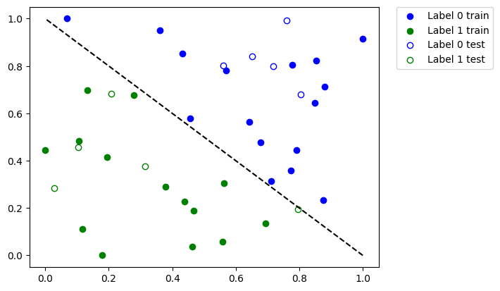
上記のプロットでは、次のようになります。
青に塗られた点は、
0というラベルの付いたトレーニングデータセットからのサンプルです。青い枠線だけの点は、
0というラベルの付いたテストデータセットからのサンプルです。緑に塗られた点は、
1というラベルの付いたトレーニングデータセットからのサンプルです。緑色の枠線だけの点は、
1というラベルの付いたテストデータセットからのサンプルです。
塗りつぶされた点を使用してモデルをトレーニングし、枠線だけの点を使用してモデルを検証します。
2. モデルをトレーニングして保存する#
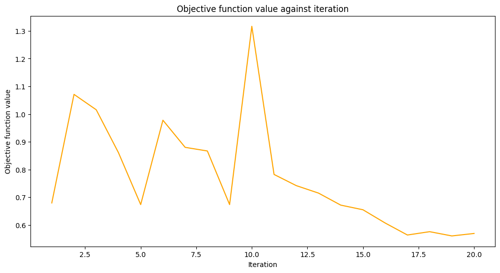
モデルを2つのステップでトレーニングします。最初のステップでは、モデルを 20 回の反復でトレーニングします。
[10]:
maxiter = 20
目的関数の値を格納するためのコールバック用の空の配列を作成します。
[11]:
objective_values = []
ニューラル・ネットワーク分類(Neural Network Classifier & Regressor)のチュートリアルのコールバック関数を再利用して、反復と目的関数の値をプロットし、いくつかの微調整を加えて、各ステップで目的値をプロットします。
[12]:
# callback function that draws a live plot when the .fit() method is called
def callback_graph(_, objective_value):
    clear_output(wait=True)
    objective_values.append(objective_value)

    plt.title("Objective function value against iteration")
    plt.xlabel("Iteration")
    plt.ylabel("Objective function value")

    stage1_len = np.min((len(objective_values), maxiter))
    stage1_x = np.linspace(1, stage1_len, stage1_len)
    stage1_y = objective_values[:stage1_len]

    stage2_len = np.max((0, len(objective_values) - maxiter))
    stage2_x = np.linspace(maxiter, maxiter + stage2_len - 1, stage2_len)
    stage2_y = objective_values[maxiter : maxiter + stage2_len]

    plt.plot(stage1_x, stage1_y, color="orange")
    plt.plot(stage2_x, stage2_y, color="purple")
    plt.show()


plt.rcParams["figure.figsize"] = (12, 6)
上記のように、 VQC モデルをトレーニングし、 maxiter パラメーターの選択された値を使用して COBYLA をオプティマイザーとして設定します。次に、モデルのパフォーマンスを評価して、モデルがどの程度適切にトレーニングされたかを確認します。次に、このモデルをファイルに保存します。2番目のステップでは、このモデルをロードし、引き続き作業します。
ここでは、最適化を開始する最初のポイントを修正するために、手動で ansatzを作成します。
[13]:
original_optimizer = COBYLA(maxiter=maxiter)

ansatz = RealAmplitudes(num_features)
initial_point = np.asarray([0.5] * ansatz.num_parameters)
モデルを作成し、sampler を先ほど作成した最初のsampler に設定します。
[14]:
original_classifier = VQC(
    ansatz=ansatz, optimizer=original_optimizer, callback=callback_graph, sampler=sampler1
)
次に、モデルをトレーニングします。
[15]:
original_classifier.fit(train_features, train_labels)
[15]:
<qiskit_machine_learning.algorithms.classifiers.vqc.VQC at 0x7fb74126db20>
トレーニングの最初のステップの後、モデルがどの程度うまく機能するかを見てみましょう。
[16]:
print("Train score", original_classifier.score(train_features, train_labels))
print("Test score ", original_classifier.score(test_features, test_labels))
Train score 0.8333333333333334
Test score  0.8
次に、モデルを保存します。任意のファイル名を選択できます。ファイル名に拡張子が指定されていない場合、 save メソッドは拡張子を追加しないことに注意してください。
[17]:
original_classifier.save("vqc_classifier.model")
3. モデルをロードし、トレーニングを続行する#
モデルをロードするには、ユーザーは対応するモデルクラスのクラスメソッド load を呼び出す必要があります。 私たちの場合は VQC です。モデルを保存した前のセクションで使用したのと同じファイル名を渡します。
[18]:
loaded_classifier = VQC.load("vqc_classifier.model")
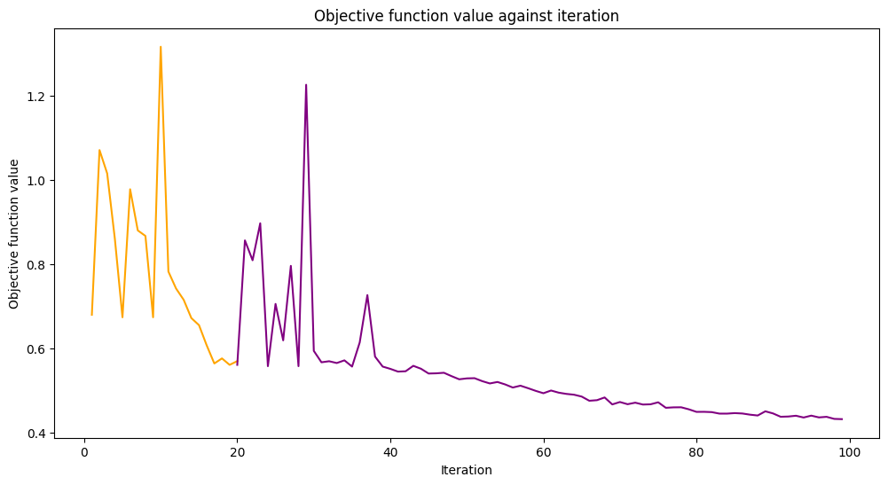
次に、このモデルをさらに別のシミュレーターで学習できるように変更したいと思います。そのために、 warm_start プロパティを設定します。このプロパティを True に設定し、再び fit() を呼び出すと、モデルは前回のフィットで得られた重みを使用して、新しいフィットを開始します。また、基礎となるネットワークの sampler プロパティを、チュートリアルの最初に作成した Sampler primitive の2番目のインスタンスに設定します。最後に、新しいオプティマイザーを作成し、 maxiter を 80 に設定して、反復処理の合計回数を 100 に設定します。
[19]:
loaded_classifier.warm_start = True
loaded_classifier.neural_network.sampler = sampler2
loaded_classifier.optimizer = COBYLA(maxiter=80)
次に、前のセクションで終了した状態からモデルのトレーニングを続けます。
[20]:
loaded_classifier.fit(train_features, train_labels)
[20]:
<qiskit_machine_learning.algorithms.classifiers.vqc.VQC at 0x7fb7411cb760>
[21]:
print("Train score", loaded_classifier.score(train_features, train_labels))
print("Test score", loaded_classifier.score(test_features, test_labels))
Train score 0.9
Test score 0.8
どのデータポイントが誤って分類されたかを見てみましょう。まず、 predict を呼び出して、トレーニング機能とテスト機能から予測値を推測します。
[22]:
train_predicts = loaded_classifier.predict(train_features)
test_predicts = loaded_classifier.predict(test_features)
データセット全体をプロットし、誤って分類されたポイントを強調表示します。
[23]:
# return plot to default figsize
plt.rcParams["figure.figsize"] = (6, 4)

plot_dataset()

# plot misclassified data points
plt.scatter(
    train_features[np.all(train_labels != train_predicts, axis=1), 0],
    train_features[np.all(train_labels != train_predicts, axis=1), 1],
    s=200,
    facecolors="none",
    edgecolors="r",
    linewidths=2,
)
plt.scatter(
    test_features[np.all(test_labels != test_predicts, axis=1), 0],
    test_features[np.all(test_labels != test_predicts, axis=1), 1],
    s=200,
    facecolors="none",
    edgecolors="r",
    linewidths=2,
)
[23]:
<matplotlib.collections.PathCollection at 0x7fb6e04c2eb0>
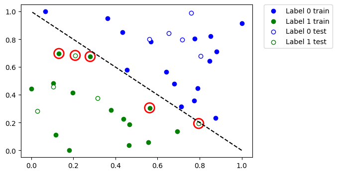
したがって、大きなデータセットまたは大きなモデルがある場合は、このチュートリアルに示すように、複数のステップでトレーニングできます。
4. PyTorchハイブリッドモデル#
ハイブリッドモデルを保存およびロードするには、TorchConnector を使用する場合、モデルの保存およびロードに関する PyTorch の推奨事項に従ってください。 詳細については、 PyTorch Connectorチュートリアル を参照してください。ここでは、短いスニペットでその方法を示しています。
この疑似的なコードを見て、アイデアを見つけてください。
# create a QNN and a hybrid model
qnn = create_qnn()
model = Net(qnn)
# ... train the model ...

# save the model
torch.save(model.state_dict(), "model.pt")

# create a new model
new_qnn = create_qnn()
loaded_model = Net(new_qnn)
loaded_model.load_state_dict(torch.load("model.pt"))
[24]:
import qiskit.tools.jupyter

%qiskit_version_table
%qiskit_copyright
Version Information
| Qiskit Software | Version |
|---|---|
qiskit-terra | 0.25.0 |
qiskit-aer | 0.13.0 |
qiskit-machine-learning | 0.7.0 |
| System information | |
| Python version | 3.8.13 |
| Python compiler | Clang 12.0.0 |
| Python build | default, Oct 19 2022 17:54:22 |
| OS | Darwin |
| CPUs | 10 |
| Memory (Gb) | 64.0 |
| Mon Jun 12 11:51:03 2023 IST | |
This code is a part of Qiskit
© Copyright IBM 2017, 2023.
This code is licensed under the Apache License, Version 2.0. You may
obtain a copy of this license in the LICENSE.txt file in the root directory
of this source tree or at http://www.apache.org/licenses/LICENSE-2.0.
Any modifications or derivative works of this code must retain this
copyright notice, and modified files need to carry a notice indicating
that they have been altered from the originals.