注釈

このページは docs/tutorials/02_neural_network_classifier_and_regressor.ipynb から生成されました。

ニューラル・ネットワーク分類器と回帰器

このチュートリアルでは、NeuralNetworkClassifier と NeuralNetworkRegressor がどのように使用されるかを示します。どちらも入力として (量子) NeuralNetwork を受け取り、特定のコンテキストでそれを活用します。どちらの場合も、利便性のためにあらかじめ設定されたバリエーション、変分量子分類器 (Variational Quantum Classifier, VQC) と変分量子回帰器 (Variational Quantum Regressor, VQR) を提供しています。チュートリアルの構成は以下の通りです。

1. 分類

   • EstimatorQNN による分類

   • SamplerQNN による分類

   • 変分量子分類器 (VQC)

2. 回帰

   • EstimatorQNN` による回帰

   • 変分量子回帰器 (VQR)

import matplotlib.pyplot as plt
import numpy as np
from IPython.display import clear_output
from qiskit import QuantumCircuit
from qiskit.circuit import Parameter
from qiskit.circuit.library import RealAmplitudes, ZZFeatureMap
from qiskit_algorithms.optimizers import COBYLA, L_BFGS_B
from qiskit_algorithms.utils import algorithm_globals

from qiskit_machine_learning.algorithms.classifiers import NeuralNetworkClassifier, VQC
from qiskit_machine_learning.algorithms.regressors import NeuralNetworkRegressor, VQR
from qiskit_machine_learning.neural_networks import SamplerQNN, EstimatorQNN
from qiskit_machine_learning.circuit.library import QNNCircuit

algorithm_globals.random_seed = 42

分類

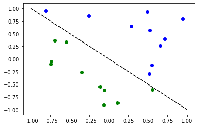
以下のアルゴリズムを説明するために、簡単な分類データセットを用意します。

num_inputs = 2
num_samples = 20
X = 2 * algorithm_globals.random.random([num_samples, num_inputs]) - 1
y01 = 1 * (np.sum(X, axis=1) >= 0)  # in { 0,  1}
y = 2 * y01 - 1  # in {-1, +1}
y_one_hot = np.zeros((num_samples, 2))
for i in range(num_samples):
    y_one_hot[i, y01[i]] = 1

for x, y_target in zip(X, y):
    if y_target == 1:
        plt.plot(x[0], x[1], "bo")
    else:
        plt.plot(x[0], x[1], "go")
plt.plot([-1, 1], [1, -1], "--", color="black")
plt.show()

EstimatorQNN による分類

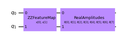
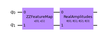
まず、 EstimatorQNN が NeuralNetworkClassifier の中でどのように分類に使われるかを示します。ここでは、 EstimatorQNN は、 \([-1, +1]\) の1次元の出力を返すことが期待されています。 これは、二値分類にしか使えないので、2つのクラスを \(\{-1, +1\}\) に割り当てます。特徴マップとansatzから簡単にパラメータ化された量子回路を合成するため、ここでは``QNNCircuit``クラスを使用します。

# construct QNN with the QNNCircuit's default ZZFeatureMap feature map and RealAmplitudes ansatz.
qc = QNNCircuit(num_qubits=2)
qc.draw(output="mpl")

量子ニューラル・ネットワークの作成

estimator_qnn = EstimatorQNN(circuit=qc)

# QNN maps inputs to [-1, +1]
estimator_qnn.forward(X[0, :], algorithm_globals.random.random(estimator_qnn.num_weights))

array([[0.23521988]])

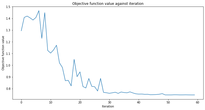
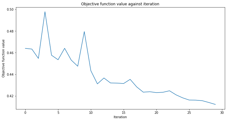
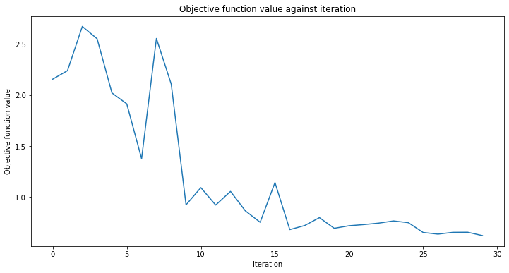
callback_graph というコールバック関数を追加します。 これはオプティマイザの反復ごとに呼び出され、現在の重みとその重みでの目的関数の値という、2つのパラメータが渡されます。 ここでは関数に、目的関数の値を配列に追加します。これによって反復と目的関数の値をプロットし、反復ごとにグラフを更新することができます。とはいえ、2つのパラメータが渡される限り、コールバック関数であなたは何でも好きなことをすることができます。

# callback function that draws a live plot when the .fit() method is called
def callback_graph(weights, obj_func_eval):
    clear_output(wait=True)
    objective_func_vals.append(obj_func_eval)
    plt.title("Objective function value against iteration")
    plt.xlabel("Iteration")
    plt.ylabel("Objective function value")
    plt.plot(range(len(objective_func_vals)), objective_func_vals)
    plt.show()

# construct neural network classifier
estimator_classifier = NeuralNetworkClassifier(
    estimator_qnn, optimizer=COBYLA(maxiter=60), callback=callback_graph
)

# create empty array for callback to store evaluations of the objective function
objective_func_vals = []
plt.rcParams["figure.figsize"] = (12, 6)

# fit classifier to data
estimator_classifier.fit(X, y)

# return to default figsize
plt.rcParams["figure.figsize"] = (6, 4)

# score classifier
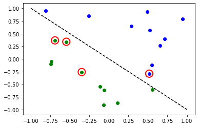
estimator_classifier.score(X, y)

0.8

# evaluate data points
y_predict = estimator_classifier.predict(X)

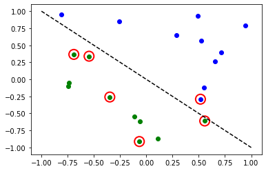
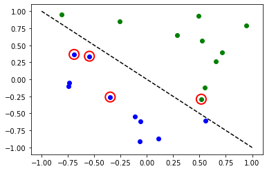
# plot results
# red == wrongly classified
for x, y_target, y_p in zip(X, y, y_predict):
    if y_target == 1:
        plt.plot(x[0], x[1], "bo")
    else:
        plt.plot(x[0], x[1], "go")
    if y_target != y_p:
        plt.scatter(x[0], x[1], s=200, facecolors="none", edgecolors="r", linewidths=2)
plt.plot([-1, 1], [1, -1], "--", color="black")
plt.show()

さて、モデルの学習が完了したら、ニューラルネットワークの重みを探索することができます。重みの数はansatzで定義されていることに注意してください。

estimator_classifier.weights

array([ 7.99142399e-01, -1.02869770e+00, -1.32131512e-04, -3.47046684e-01,
        1.13636802e+00,  6.56831727e-01,  2.17902158e+00, -1.08678332e+00])

SamplerQNN による分類

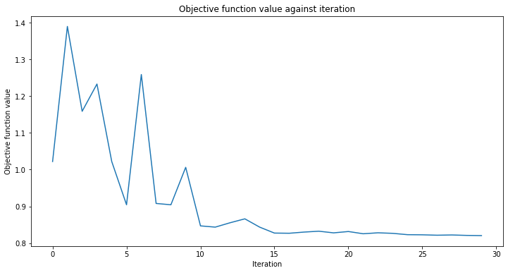
次に、 SamplerQNN が NeuralNetworkClassifier の中でどのように分類に使われるかを示します。ここでは、 SamplerQNN は、 \(d\) -次元の確率ベクトルを出力として返すことが期待されます。ここで \(d\) はクラス数です。基礎となる Sampler primitiveはビット列の準分布を返すので、測定されたビット列から異なるクラスへのマッピングを定義するだけでよいのです。2値分類には、パリティーマッピングを用います。ここでも QNNCircuit クラスを使って、任意の特徴量マップとansatzからパラメーター化された量子回路を設定することができます。

# construct a quantum circuit from the default ZZFeatureMap feature map and a customized RealAmplitudes ansatz
qc = QNNCircuit(ansatz=RealAmplitudes(num_inputs, reps=1))
qc.draw(output="mpl")

# parity maps bitstrings to 0 or 1
def parity(x):
    return "{:b}".format(x).count("1") % 2


output_shape = 2  # corresponds to the number of classes, possible outcomes of the (parity) mapping.

# construct QNN
sampler_qnn = SamplerQNN(
    circuit=qc,
    interpret=parity,
    output_shape=output_shape,
)

# construct classifier
sampler_classifier = NeuralNetworkClassifier(
    neural_network=sampler_qnn, optimizer=COBYLA(maxiter=30), callback=callback_graph
)

# create empty array for callback to store evaluations of the objective function
objective_func_vals = []
plt.rcParams["figure.figsize"] = (12, 6)

# fit classifier to data
sampler_classifier.fit(X, y01)

# return to default figsize
plt.rcParams["figure.figsize"] = (6, 4)

# score classifier
sampler_classifier.score(X, y01)

0.7

# evaluate data points
y_predict = sampler_classifier.predict(X)

# plot results
# red == wrongly classified
for x, y_target, y_p in zip(X, y01, y_predict):
    if y_target == 1:
        plt.plot(x[0], x[1], "bo")
    else:
        plt.plot(x[0], x[1], "go")
    if y_target != y_p:
        plt.scatter(x[0], x[1], s=200, facecolors="none", edgecolors="r", linewidths=2)
plt.plot([-1, 1], [1, -1], "--", color="black")
plt.show()

繰り返しになりますが、モデルの学習が完了したら、重みを見ることができます。Ansatzで明示的に reps=1 を設定しているので、前のモデルよりもパラメーターが少なくなっていることがわかります。

sampler_classifier.weights

array([ 1.67198565,  0.46045402, -0.93462862, -0.95266092])

変分量子分類器 (VQC)

VQC は、SamplerQNN を用いた NeuralNetworkClassifier の特別なバリエーションです。VQC は、パリティー・マッピング（または複数のクラスへの拡張）を適用して、ビット列から分類にマッピングし、その結果、確率ベクトルが得られ、ワンショットでエンコードされた結果として解釈されます。デフォルトでは、 CrossEntropyLoss 関数を適用します。この関数は、ワンショットでエンコードされたフォーマットで与えられたラベルを想定しており、そのフォーマットでも予測値を返します。

# construct feature map, ansatz, and optimizer
feature_map = ZZFeatureMap(num_inputs)
ansatz = RealAmplitudes(num_inputs, reps=1)

# construct variational quantum classifier
vqc = VQC(
    feature_map=feature_map,
    ansatz=ansatz,
    loss="cross_entropy",
    optimizer=COBYLA(maxiter=30),
    callback=callback_graph,
)

# create empty array for callback to store evaluations of the objective function
objective_func_vals = []
plt.rcParams["figure.figsize"] = (12, 6)

# fit classifier to data
vqc.fit(X, y_one_hot)

# return to default figsize
plt.rcParams["figure.figsize"] = (6, 4)

# score classifier
vqc.score(X, y_one_hot)

0.8

# evaluate data points
y_predict = vqc.predict(X)

# plot results
# red == wrongly classified
for x, y_target, y_p in zip(X, y_one_hot, y_predict):
    if y_target[0] == 1:
        plt.plot(x[0], x[1], "bo")
    else:
        plt.plot(x[0], x[1], "go")
    if not np.all(y_target == y_p):
        plt.scatter(x[0], x[1], s=200, facecolors="none", edgecolors="r", linewidths=2)
plt.plot([-1, 1], [1, -1], "--", color="black")
plt.show()

VQC を使用した複数のクラス

この節では，3つのクラスのサンプルを含む人工データセットを生成し，このデータセットを分類するモデルをどのように学習するかを示します。この例は，機械学習におけるより興味深い問題への取り組み方を示しています。もちろん、学習時間を短くするために、小さなデータセットを用意します。SciKit-Learnの make_classification を用いてデータセットを生成します。データセットには10個のサンプル、2個の特徴量がありますが、これはデータセットをきれいにプロットできることと、冗長な特徴はなく、これらは他の特徴量の組み合わせとして生成されることを意味しています。また、データセットには3つの異なるクラスがあり、それぞれのクラスには1種類のセントロイドがあります。クラス分離は、分類問題を緩和するために、デフォルト値の 1.0 から少し増やして 2.0 に設定しました。

データセットが生成されると、その機能を [0, 1] の範囲に拡大します。

from sklearn.datasets import make_classification
from sklearn.preprocessing import MinMaxScaler

X, y = make_classification(
    n_samples=10,
    n_features=2,
    n_classes=3,
    n_redundant=0,
    n_clusters_per_class=1,
    class_sep=2.0,
    random_state=algorithm_globals.random_seed,
)
X = MinMaxScaler().fit_transform(X)

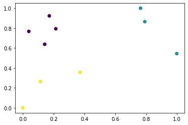
データセットがどのように見えるか見てみましょう。

plt.scatter(X[:, 0], X[:, 1], c=y)

<matplotlib.collections.PathCollection at 0x7fd5e072c250>

また、ラベルを変換してカテゴリー化することもできます。

y_cat = np.empty(y.shape, dtype=str)
y_cat[y == 0] = "A"
y_cat[y == 1] = "B"
y_cat[y == 2] = "C"
print(y_cat)

['A' 'A' 'B' 'C' 'C' 'A' 'B' 'B' 'A' 'C']

前の例と同様に VQC のインスタンスを作成しますが、今回は最小限のパラメーターを渡します。特徴量マップとansatzの代わりに、データセットの特徴量数に等しい量子ビットの数、学習時間を短縮するための低い反復回数のオプティマイザー、量子インスタンス、そして進捗を確認するためのコールバックを渡します。

vqc = VQC(
    num_qubits=2,
    optimizer=COBYLA(maxiter=30),
    callback=callback_graph,
)

前の例と同じ方法でトレーニング・プロセスを開始します。

# create empty array for callback to store evaluations of the objective function
objective_func_vals = []
plt.rcParams["figure.figsize"] = (12, 6)

# fit classifier to data
vqc.fit(X, y_cat)

# return to default figsize
plt.rcParams["figure.figsize"] = (6, 4)

# score classifier
vqc.score(X, y_cat)

0.9

反復回数が少なかったにもかかわらず、私たちはかなり良いスコアを達成しました。 predict メソッドの出力を確認し、出力と基本となる真の値と比較してみましょう。

predict = vqc.predict(X)
print(f"Predicted labels: {predict}")
print(f"Ground truth:     {y_cat}")

Predicted labels: ['A' 'A' 'B' 'C' 'C' 'A' 'B' 'B' 'A' 'B']
Ground truth:     ['A' 'A' 'B' 'C' 'C' 'A' 'B' 'B' 'A' 'C']

回帰

以下のアルゴリズムを説明するために、簡単な回帰データセットを用意します。

num_samples = 20
eps = 0.2
lb, ub = -np.pi, np.pi
X_ = np.linspace(lb, ub, num=50).reshape(50, 1)
f = lambda x: np.sin(x)

X = (ub - lb) * algorithm_globals.random.random([num_samples, 1]) + lb
y = f(X[:, 0]) + eps * (2 * algorithm_globals.random.random(num_samples) - 1)

plt.plot(X_, f(X_), "r--")
plt.plot(X, y, "bo")
plt.show()

EstimatorQNN` による回帰

ここでは、 \([-1, +1]\) の値を返す EstimatorQNN を使った回帰に限定します。もっと複雑で多次元のモデルを SamplerQNN をベースにして構築することもできますが、このチュートリアルの範囲を超えています。

# construct simple feature map
param_x = Parameter("x")
feature_map = QuantumCircuit(1, name="fm")
feature_map.ry(param_x, 0)

# construct simple ansatz
param_y = Parameter("y")
ansatz = QuantumCircuit(1, name="vf")
ansatz.ry(param_y, 0)

# construct a circuit
qc = QNNCircuit(feature_map=feature_map, ansatz=ansatz)

# construct QNN
regression_estimator_qnn = EstimatorQNN(circuit=qc)

# construct the regressor from the neural network
regressor = NeuralNetworkRegressor(
    neural_network=regression_estimator_qnn,
    loss="squared_error",
    optimizer=L_BFGS_B(maxiter=5),
    callback=callback_graph,
)

# create empty array for callback to store evaluations of the objective function
objective_func_vals = []
plt.rcParams["figure.figsize"] = (12, 6)

# fit to data
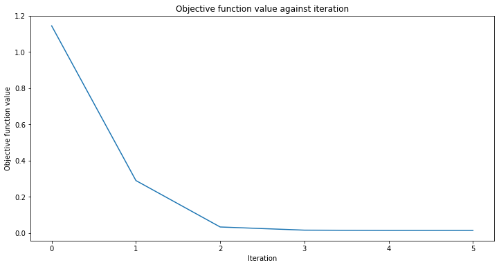
regressor.fit(X, y)

# return to default figsize
plt.rcParams["figure.figsize"] = (6, 4)

# score the result
regressor.score(X, y)

0.9769994291935522

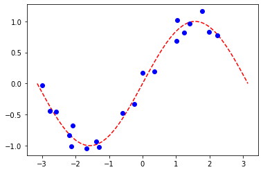
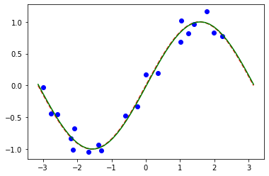
# plot target function
plt.plot(X_, f(X_), "r--")

# plot data
plt.plot(X, y, "bo")

# plot fitted line
y_ = regressor.predict(X_)
plt.plot(X_, y_, "g-")
plt.show()

分類モデルと同様に、モデルの対応するプロパティーを問い合わせることで、学習済み重みの配列を取得することができます。このモデルでは，上記の param_y として定義されたパラメーターを1つだけ持ちます。

regressor.weights

array([-1.58870599])

変分量子回帰器 (VQR) による回帰

VQR は、分類用の VQC と同様に、EstimatorQNN を用いた NeuralNetworkRegressor の特別な改良版です。デフォルトでは、予測値と目標値の間の平均二乗誤差を最小化するために、 L2Loss 関数を考慮します。

vqr = VQR(
    feature_map=feature_map,
    ansatz=ansatz,
    optimizer=L_BFGS_B(maxiter=5),
    callback=callback_graph,
)

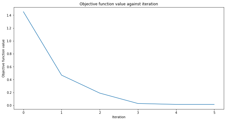
# create empty array for callback to store evaluations of the objective function
objective_func_vals = []
plt.rcParams["figure.figsize"] = (12, 6)

# fit regressor
vqr.fit(X, y)

# return to default figsize
plt.rcParams["figure.figsize"] = (6, 4)

# score result
vqr.score(X, y)

0.9769955693935385

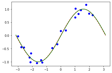
# plot target function
plt.plot(X_, f(X_), "r--")

# plot data
plt.plot(X, y, "bo")

# plot fitted line
y_ = vqr.predict(X_)
plt.plot(X_, y_, "g-")
plt.show()

import qiskit.tools.jupyter

%qiskit_version_table
%qiskit_copyright

Version Information

Qiskit Software	Version
qiskit-terra	0.24.0
qiskit-aer	0.12.0
qiskit-ignis	0.6.0
qiskit-ibmq-provider	0.20.2
qiskit	0.43.0
qiskit-machine-learning	0.7.0
System information
Python version	3.8.8
Python compiler	Clang 10.0.0
Python build	default, Apr 13 2021 12:59:45
OS	Darwin
CPUs	8
Memory (Gb)	32.0
Tue Jun 13 16:39:30 2023 CEST

This code is a part of Qiskit

© Copyright IBM 2017, 2023.

This code is licensed under the Apache License, Version 2.0. You may
obtain a copy of this license in the LICENSE.txt file in the root directory
of this source tree or at http://www.apache.org/licenses/LICENSE-2.0.

Any modifications or derivative works of this code must retain this
copyright notice, and modified files need to carry a notice indicating
that they have been altered from the originals.