注釈
このページは docs/tutorials/05_torch_connector.ipynb から生成されました。
Torch コネクターおよびハイブリッド QNN#
このチュートリアルでは、TorchConnector クラスを紹介します。そして、 TorchConnector が Qiskit 機械学習から PyTorch ワークフローに NeuralNetwork を自然に統合する方法を示します。 TorchConnector は NeuralNetwork を受け取り、PyTorchの Module として利用できるようにします。 得られたモジュールは、PyTorchの古典アーキテクチャーにシームレスに組み込むことができ、追加の考慮事項なしに一緒に学習することができます。 また、新しい ハイブリッド量子古典 機械学習アーキテクチャーの開発とテストを可能にします。
目次:#
パート 1: 簡単な分類と回帰
このチュートリアルの最初の部分は、PyTorchの自動微分エンジン( torch.autograd、 リンク) を使用して簡単な分類と回帰タスクのための量子ニューラルネットワークを学習させる方法を示しています。
分類
PyTorch と
EstimatorQNNによる分類PyTorch と
SamplerQNNを用いた分類
回帰
PyTorchと
EstimatorQNNによる回帰
パート 2: MNIST 分類、ハイブリッドQNN
このチュートリアルの 2 番目の部分では、ハイブリッドの量子古典的な方法で MNIST データを分類するため、 (量子) NeuralNetwork をターゲットの PyTorch ワークフロー ( この場合は、典型的な CNN アーキテクチャー) に組み込む方法を説明しています。
[1]:
# Necessary imports

import numpy as np
import matplotlib.pyplot as plt

from torch import Tensor
from torch.nn import Linear, CrossEntropyLoss, MSELoss
from torch.optim import LBFGS

from qiskit import QuantumCircuit
from qiskit.circuit import Parameter
from qiskit.circuit.library import RealAmplitudes, ZZFeatureMap
from qiskit_algorithms.utils import algorithm_globals
from qiskit_machine_learning.neural_networks import SamplerQNN, EstimatorQNN
from qiskit_machine_learning.connectors import TorchConnector

# Set seed for random generators
algorithm_globals.random_seed = 42
パート 1: 簡単な分類と回帰#
1. 分類#
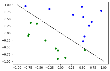
最初に、TorchConnector が PyTorch の自動微分エンジンを使用して、分類タスクを解決するために 量子 NeuralNetwork を学習させる方法を示します。 これを示すために、ランダムに生成されたデータセットに対し バイナリ分類 を実行します。
[2]:
# Generate random dataset

# Select dataset dimension (num_inputs) and size (num_samples)
num_inputs = 2
num_samples = 20

# Generate random input coordinates (X) and binary labels (y)
X = 2 * algorithm_globals.random.random([num_samples, num_inputs]) - 1
y01 = 1 * (np.sum(X, axis=1) >= 0)  # in { 0,  1}, y01 will be used for SamplerQNN example
y = 2 * y01 - 1  # in {-1, +1}, y will be used for EstimatorQNN example

# Convert to torch Tensors
X_ = Tensor(X)
y01_ = Tensor(y01).reshape(len(y)).long()
y_ = Tensor(y).reshape(len(y), 1)

# Plot dataset
for x, y_target in zip(X, y):
    if y_target == 1:
        plt.plot(x[0], x[1], "bo")
    else:
        plt.plot(x[0], x[1], "go")
plt.plot([-1, 1], [1, -1], "--", color="black")
plt.show()
A. PyTorch と EstimatorQNN による分類#
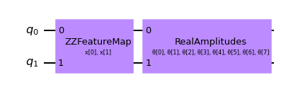
EstimatorQNN と PyTorch のリンクは比較的簡単です。ここでは、特徴量マップとansatzから構築された EstimatorQNN を使って説明します。
[3]:
# Set up a circuit
feature_map = ZZFeatureMap(num_inputs)
ansatz = RealAmplitudes(num_inputs)
qc = QuantumCircuit(num_inputs)
qc.compose(feature_map, inplace=True)
qc.compose(ansatz, inplace=True)
qc.draw("mpl")
[3]:
[4]:
# Setup QNN
qnn1 = EstimatorQNN(
    circuit=qc, input_params=feature_map.parameters, weight_params=ansatz.parameters
)

# Set up PyTorch module
# Note: If we don't explicitly declare the initial weights
# they are chosen uniformly at random from [-1, 1].
initial_weights = 0.1 * (2 * algorithm_globals.random.random(qnn1.num_weights) - 1)
model1 = TorchConnector(qnn1, initial_weights=initial_weights)
print("Initial weights: ", initial_weights)
Initial weights:  [-0.01256962  0.06653564  0.04005302 -0.03752667  0.06645196  0.06095287
 -0.02250432 -0.04233438]
[5]:
# Test with a single input
model1(X_[0, :])
[5]:
tensor([-0.3285], grad_fn=<_TorchNNFunctionBackward>)
オプティマイザー#
あらゆる機械学習モデルを学習させる上でオプティマイザーの選択は、学習の成果を決定する上で非常に重要です。 TorchConnector を使用する場合、[torch.optim] パッケージ (リンク) で定義されているすべてのオプティマイザー・アルゴリズムを使用できます。 一般的な機械学習アーキテクチャーで使用される最も有名なアルゴリズムには、Adam、SGD、または Adagrad があります。 しかし、このチュートリアルではL-BFGSアルゴリズム(torch.optim.LBFGS)を使用します。 数値最適化のための最もよく知られている2次最適化アルゴリズムの1つです。
損失関数#
損失関数については、交差エントロピー や 平均二乗誤差 損失といった、 torch.nn パッケージからPyTorchの事前定義モジュールを利用することができます。
💡 解説 : 古典機械学習において一般的な経験則は、分類タスクに交差エントロピー損失を適用し、回帰タスクにMSE損失を適用することです。 しかし、この推奨は、分類ネットワークの出力が \([0, 1]\) 範囲 (通常は Softmax レイヤーを介して達成) の分類確率値であることを前提としています。 EstimatorQNN の以下の例にはそのようなレイヤーが含まれないため、また、出力にマッピングを適用することもない (次のセクションでは SamplerQNN を使用したパリティ・マッピングの例を示します) ため、QNNの出力は、 \([-1, 1]\) の範囲で任意の値を取ることができます。 因みに、これが、この特定の例でMSELossを一般的でないのにも関わらず分類に使用している理由です(ただし、さまざまな損失関数を試して、学習結果にどのような影響を与えるかを確認することをお勧めします)。
[6]:
# Define optimizer and loss
optimizer = LBFGS(model1.parameters())
f_loss = MSELoss(reduction="sum")

# Start training
model1.train()  # set model to training mode


# Note from (https://pytorch.org/docs/stable/optim.html):
# Some optimization algorithms such as LBFGS need to
# reevaluate the function multiple times, so you have to
# pass in a closure that allows them to recompute your model.
# The closure should clear the gradients, compute the loss,
# and return it.
def closure():
    optimizer.zero_grad()  # Initialize/clear gradients
    loss = f_loss(model1(X_), y_)  # Evaluate loss function
    loss.backward()  # Backward pass
    print(loss.item())  # Print loss
    return loss


# Run optimizer step4
optimizer.step(closure)
25.535646438598633
22.696760177612305
20.039228439331055
19.687908172607422
19.267208099365234
19.025373458862305
18.154708862304688
17.337854385375977
19.082578659057617
17.073287963867188
16.21839141845703
14.992582321166992
14.929339408874512
14.914533615112305
14.907636642456055
14.902364730834961
14.902134895324707
14.90211009979248
14.902111053466797
[6]:
tensor(25.5356, grad_fn=<MseLossBackward0>)
[7]:
# Evaluate model and compute accuracy
model1.eval()
y_predict = []
for x, y_target in zip(X, y):
    output = model1(Tensor(x))
    y_predict += [np.sign(output.detach().numpy())[0]]

print("Accuracy:", sum(y_predict == y) / len(y))

# Plot results
# red == wrongly classified
for x, y_target, y_p in zip(X, y, y_predict):
    if y_target == 1:
        plt.plot(x[0], x[1], "bo")
    else:
        plt.plot(x[0], x[1], "go")
    if y_target != y_p:
        plt.scatter(x[0], x[1], s=200, facecolors="none", edgecolors="r", linewidths=2)
plt.plot([-1, 1], [1, -1], "--", color="black")
plt.show()
Accuracy: 0.8
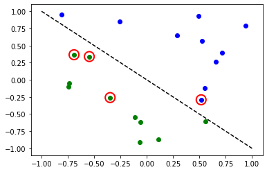
赤い丸は、誤って分類されたデータポイントを示します。
B. PyTorch と SamplerQNN を用いた分類#
SamplerQNN を PyTorch にリンクするには、EstimatorQNN` よりも少し注意が必要です。正しい設定がなければ、誤差逆伝播はできません。
特に、ネットワークのフォワードパス(sparse=False) に確率の密な配列を返していることを確認する必要があります。 このパラメーターはデフォルトでは False に設定されているため、変更されていないことを確認する必要があります。
⚠️ 注意: カスタムのinterpret関数を定義した場合 (例: parity) 、期待する出力の形状 (例: 2) を明示的に指定する必要があります。 SamplerQNN の初期設定に関する詳細は、 公式のQiskitドキュメンテーション を参照してください。
[8]:
# Define feature map and ansatz
feature_map = ZZFeatureMap(num_inputs)
ansatz = RealAmplitudes(num_inputs, entanglement="linear", reps=1)

# Define quantum circuit of num_qubits = input dim
# Append feature map and ansatz
qc = QuantumCircuit(num_inputs)
qc.compose(feature_map, inplace=True)
qc.compose(ansatz, inplace=True)

# Define SamplerQNN and initial setup
parity = lambda x: "{:b}".format(x).count("1") % 2  # optional interpret function
output_shape = 2  # parity = 0, 1
qnn2 = SamplerQNN(
    circuit=qc,
    input_params=feature_map.parameters,
    weight_params=ansatz.parameters,
    interpret=parity,
    output_shape=output_shape,
)

# Set up PyTorch module
# Reminder: If we don't explicitly declare the initial weights
# they are chosen uniformly at random from [-1, 1].
initial_weights = 0.1 * (2 * algorithm_globals.random.random(qnn2.num_weights) - 1)
print("Initial weights: ", initial_weights)
model2 = TorchConnector(qnn2, initial_weights)
Initial weights: [ 0.0364991 -0.0720495 -0.06001836 -0.09852755]
オプティマイザーと損失関数の選択について思い出すには、このセクション に戻ってください。
[9]:
# Define model, optimizer, and loss
optimizer = LBFGS(model2.parameters())
f_loss = CrossEntropyLoss()  # Our output will be in the [0,1] range

# Start training
model2.train()

# Define LBFGS closure method (explained in previous section)
def closure():
    optimizer.zero_grad(set_to_none=True)  # Initialize gradient
    loss = f_loss(model2(X_), y01_)  # Calculate loss
    loss.backward()  # Backward pass

    print(loss.item())  # Print loss
    return loss


# Run optimizer (LBFGS requires closure)
optimizer.step(closure);
0.6925069093704224
0.6881508231163025
0.6516683101654053
0.6485998034477234
0.6394743919372559
0.7057444453239441
0.669085681438446
0.766187310218811
0.7188469171524048
0.7919709086418152
0.7598814964294434
0.7028256058692932
0.7486447095870972
0.6890242695808411
0.7760348916053772
0.7892935276031494
0.7556288242340088
0.7058126330375671
0.7203161716461182
0.7030722498893738
[10]:
# Evaluate model and compute accuracy
model2.eval()
y_predict = []
for x in X:
    output = model2(Tensor(x))
    y_predict += [np.argmax(output.detach().numpy())]

print("Accuracy:", sum(y_predict == y01) / len(y01))

# plot results
# red == wrongly classified
for x, y_target, y_ in zip(X, y01, y_predict):
    if y_target == 1:
        plt.plot(x[0], x[1], "bo")
    else:
        plt.plot(x[0], x[1], "go")
    if y_target != y_:
        plt.scatter(x[0], x[1], s=200, facecolors="none", edgecolors="r", linewidths=2)
plt.plot([-1, 1], [1, -1], "--", color="black")
plt.show()
Accuracy: 0.5
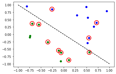
赤い丸は、誤って分類されたデータポイントを示します。
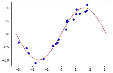
2. 回帰#
EstimatorQNN に基づいたモデルを使用して、回帰タスクの実行方法を説明します。 今回選択されたデータセットは、正弦波に沿ってランダムに生成されたものです。
[11]:
# Generate random dataset

num_samples = 20
eps = 0.2
lb, ub = -np.pi, np.pi
f = lambda x: np.sin(x)

X = (ub - lb) * algorithm_globals.random.random([num_samples, 1]) + lb
y = f(X) + eps * (2 * algorithm_globals.random.random([num_samples, 1]) - 1)
plt.plot(np.linspace(lb, ub), f(np.linspace(lb, ub)), "r--")
plt.plot(X, y, "bo")
plt.show()
A. PyTorchと EstimatorQNN による回帰#
ネットワーク定義と学習ループは、 EstimatorQNN を使用した分類タスクのものと類似しています。 この場合、独自の特徴マップとansatzを定義しますが、少し違った方法で定義してみましょう。
[12]:
# Construct simple feature map
param_x = Parameter("x")
feature_map = QuantumCircuit(1, name="fm")
feature_map.ry(param_x, 0)

# Construct simple parameterized ansatz
param_y = Parameter("y")
ansatz = QuantumCircuit(1, name="vf")
ansatz.ry(param_y, 0)

qc = QuantumCircuit(1)
qc.compose(feature_map, inplace=True)
qc.compose(ansatz, inplace=True)

# Construct QNN
qnn3 = EstimatorQNN(circuit=qc, input_params=[param_x], weight_params=[param_y])

# Set up PyTorch module
# Reminder: If we don't explicitly declare the initial weights
# they are chosen uniformly at random from [-1, 1].
initial_weights = 0.1 * (2 * algorithm_globals.random.random(qnn3.num_weights) - 1)
model3 = TorchConnector(qnn3, initial_weights)
オプティマイザーと損失関数の選択について思い出すには、このセクション に戻ってください。
[13]:
# Define optimizer and loss function
optimizer = LBFGS(model3.parameters())
f_loss = MSELoss(reduction="sum")

# Start training
model3.train()  # set model to training mode

# Define objective function
def closure():
    optimizer.zero_grad(set_to_none=True)  # Initialize gradient
    loss = f_loss(model3(Tensor(X)), Tensor(y))  # Compute batch loss
    loss.backward()  # Backward pass
    print(loss.item())  # Print loss
    return loss


# Run optimizer
optimizer.step(closure)
14.947757720947266
2.948650360107422
8.952412605285645
0.37905153632164
0.24995625019073486
0.2483610212802887
0.24835753440856934
[13]:
tensor(14.9478, grad_fn=<MseLossBackward0>)
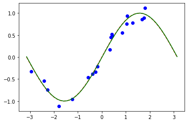
[14]:
# Plot target function
plt.plot(np.linspace(lb, ub), f(np.linspace(lb, ub)), "r--")

# Plot data
plt.plot(X, y, "bo")

# Plot fitted line
model3.eval()
y_ = []
for x in np.linspace(lb, ub):
    output = model3(Tensor([x]))
    y_ += [output.detach().numpy()[0]]
plt.plot(np.linspace(lb, ub), y_, "g-")
plt.show()
パート 2: MNIST 分類、ハイブリッドQNN#
2番目の部分では、TorchConnector を使用したハイブリッドの量子古典的なニューラルネットワークの活用方法を示します。 より複雑な画像分類タスクをMNISTの手書きの数字データセットで実行します。
ハイブリッドの量子古典ニューラルネットワークの詳細(TorchConnector の前)については、Qiskit Textbook の対応するセクションを参照してください。
[15]:
# Additional torch-related imports
import torch
from torch import cat, no_grad, manual_seed
from torch.utils.data import DataLoader
from torchvision import datasets, transforms
import torch.optim as optim
from torch.nn import (
    Module,
    Conv2d,
    Linear,
    Dropout2d,
    NLLLoss,
    MaxPool2d,
    Flatten,
    Sequential,
    ReLU,
)
import torch.nn.functional as F
ステップ 1: 学習とテスト用のデータ・ローダーの定義#
torchvision API を利用して、 MNIST データセット のサブセットを直接ロードし、学習とテストのための DataLoader (リンク) を定義します。
[16]:
# Train Dataset
# -------------

# Set train shuffle seed (for reproducibility)
manual_seed(42)

batch_size = 1
n_samples = 100  # We will concentrate on the first 100 samples

# Use pre-defined torchvision function to load MNIST train data
X_train = datasets.MNIST(
    root="./data", train=True, download=True, transform=transforms.Compose([transforms.ToTensor()])
)

# Filter out labels (originally 0-9), leaving only labels 0 and 1
idx = np.append(
    np.where(X_train.targets == 0)[0][:n_samples], np.where(X_train.targets == 1)[0][:n_samples]
)
X_train.data = X_train.data[idx]
X_train.targets = X_train.targets[idx]

# Define torch dataloader with filtered data
train_loader = DataLoader(X_train, batch_size=batch_size, shuffle=True)
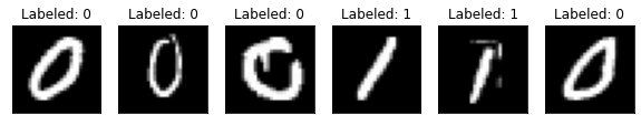
簡単な可視化を実行すると、学習のデータセットは手書きの0と1の画像で構成されていることがわかります。
[17]:
n_samples_show = 6

data_iter = iter(train_loader)
fig, axes = plt.subplots(nrows=1, ncols=n_samples_show, figsize=(10, 3))

while n_samples_show > 0:
    images, targets = data_iter.__next__()

    axes[n_samples_show - 1].imshow(images[0, 0].numpy().squeeze(), cmap="gray")
    axes[n_samples_show - 1].set_xticks([])
    axes[n_samples_show - 1].set_yticks([])
    axes[n_samples_show - 1].set_title("Labeled: {}".format(targets[0].item()))

    n_samples_show -= 1
[18]:
# Test Dataset
# -------------

# Set test shuffle seed (for reproducibility)
# manual_seed(5)

n_samples = 50

# Use pre-defined torchvision function to load MNIST test data
X_test = datasets.MNIST(
    root="./data", train=False, download=True, transform=transforms.Compose([transforms.ToTensor()])
)

# Filter out labels (originally 0-9), leaving only labels 0 and 1
idx = np.append(
    np.where(X_test.targets == 0)[0][:n_samples], np.where(X_test.targets == 1)[0][:n_samples]
)
X_test.data = X_test.data[idx]
X_test.targets = X_test.targets[idx]

# Define torch dataloader with filtered data
test_loader = DataLoader(X_test, batch_size=batch_size, shuffle=True)
ステップ 2: QNNとハイブリッド・モデルの定義#
この2番目のステップは、 TorchConnector の実力を示します。 量子ニューラルネットワーク層を定義した後 (この場合は EstimatorQNN) 、torchコネクターを TorchConnector(qnn) として初期化することで、torch Module のレイヤーに埋め込むことができます。
⚠️ 注意: ハイブリッド・モデルで、適切な勾配バックプロパゲーションを行うためには、QNNの初期化中に、初期パラメーター input_gradients を TRUE に設定する必要があります。
[19]:
# Define and create QNN
def create_qnn():
    feature_map = ZZFeatureMap(2)
    ansatz = RealAmplitudes(2, reps=1)
    qc = QuantumCircuit(2)
    qc.compose(feature_map, inplace=True)
    qc.compose(ansatz, inplace=True)

    # REMEMBER TO SET input_gradients=True FOR ENABLING HYBRID GRADIENT BACKPROP
    qnn = EstimatorQNN(
        circuit=qc,
        input_params=feature_map.parameters,
        weight_params=ansatz.parameters,
        input_gradients=True,
    )
    return qnn


qnn4 = create_qnn()
[20]:
# Define torch NN module


class Net(Module):
    def __init__(self, qnn):
        super().__init__()
        self.conv1 = Conv2d(1, 2, kernel_size=5)
        self.conv2 = Conv2d(2, 16, kernel_size=5)
        self.dropout = Dropout2d()
        self.fc1 = Linear(256, 64)
        self.fc2 = Linear(64, 2)  # 2-dimensional input to QNN
        self.qnn = TorchConnector(qnn)  # Apply torch connector, weights chosen
        # uniformly at random from interval [-1,1].
        self.fc3 = Linear(1, 1)  # 1-dimensional output from QNN

    def forward(self, x):
        x = F.relu(self.conv1(x))
        x = F.max_pool2d(x, 2)
        x = F.relu(self.conv2(x))
        x = F.max_pool2d(x, 2)
        x = self.dropout(x)
        x = x.view(x.shape[0], -1)
        x = F.relu(self.fc1(x))
        x = self.fc2(x)
        x = self.qnn(x)  # apply QNN
        x = self.fc3(x)
        return cat((x, 1 - x), -1)


model4 = Net(qnn4)
ステップ 3: 学習#
[21]:
# Define model, optimizer, and loss function
optimizer = optim.Adam(model4.parameters(), lr=0.001)
loss_func = NLLLoss()

# Start training
epochs = 10  # Set number of epochs
loss_list = []  # Store loss history
model4.train()  # Set model to training mode

for epoch in range(epochs):
    total_loss = []
    for batch_idx, (data, target) in enumerate(train_loader):
        optimizer.zero_grad(set_to_none=True)  # Initialize gradient
        output = model4(data)  # Forward pass
        loss = loss_func(output, target)  # Calculate loss
        loss.backward()  # Backward pass
        optimizer.step()  # Optimize weights
        total_loss.append(loss.item())  # Store loss
    loss_list.append(sum(total_loss) / len(total_loss))
    print("Training [{:.0f}%]\tLoss: {:.4f}".format(100.0 * (epoch + 1) / epochs, loss_list[-1]))
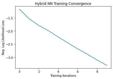
Training [10%]  Loss: -1.1630
Training [20%]  Loss: -1.5294
Training [30%]  Loss: -1.7855
Training [40%]  Loss: -1.9863
Training [50%]  Loss: -2.2257
Training [60%]  Loss: -2.4513
Training [70%]  Loss: -2.6758
Training [80%]  Loss: -2.8832
Training [90%]  Loss: -3.1006
Training [100%] Loss: -3.3061
[22]:
# Plot loss convergence
plt.plot(loss_list)
plt.title("Hybrid NN Training Convergence")
plt.xlabel("Training Iterations")
plt.ylabel("Neg. Log Likelihood Loss")
plt.show()
次に、トレーニング済みモデルを保存して、ハイブリッドモデルを保存し、後で推論に再利用する方法を示します。ハイブリッドモデルを保存およびロードにおいて、TorchConnector を使用する場合、モデルの保存およびロードに関する PyTorch の推奨事項に従ってください。
[23]:
torch.save(model4.state_dict(), "model4.pt")
ステップ 4: 評価#
モデルを再作成し、以前に保存したファイルから状態をロードすることから始めます。別のシミュレーターまたは実際のハードウェアを使用してQNNレイヤーを作成します。したがって、クラウドで利用可能な実際のハードウェアでモデルをトレーニングしてから、推論にシミュレーターまたはその逆を使用できます。簡単にするために、上記と同じ方法で新しい量子ニューラルネットワークを作成します。
[24]:
qnn5 = create_qnn()
model5 = Net(qnn5)
model5.load_state_dict(torch.load("model4.pt"))
[24]:
<All keys matched successfully>
[25]:
model5.eval()  # set model to evaluation mode
with no_grad():

    correct = 0
    for batch_idx, (data, target) in enumerate(test_loader):
        output = model5(data)
        if len(output.shape) == 1:
            output = output.reshape(1, *output.shape)

        pred = output.argmax(dim=1, keepdim=True)
        correct += pred.eq(target.view_as(pred)).sum().item()

        loss = loss_func(output, target)
        total_loss.append(loss.item())

    print(
        "Performance on test data:\n\tLoss: {:.4f}\n\tAccuracy: {:.1f}%".format(
            sum(total_loss) / len(total_loss), correct / len(test_loader) / batch_size * 100
        )
    )
Performance on test data:
        Loss: -3.3585
        Accuracy: 100.0%
[26]:
# Plot predicted labels

n_samples_show = 6
count = 0
fig, axes = plt.subplots(nrows=1, ncols=n_samples_show, figsize=(10, 3))

model5.eval()
with no_grad():
    for batch_idx, (data, target) in enumerate(test_loader):
        if count == n_samples_show:
            break
        output = model5(data[0:1])
        if len(output.shape) == 1:
            output = output.reshape(1, *output.shape)

        pred = output.argmax(dim=1, keepdim=True)

        axes[count].imshow(data[0].numpy().squeeze(), cmap="gray")

        axes[count].set_xticks([])
        axes[count].set_yticks([])
        axes[count].set_title("Predicted {}".format(pred.item()))

        count += 1
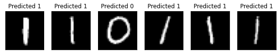
🎉🎉🎉🎉🎉 これで、Qiskit 機械学習を使用して、独自のハイブリッド・データセットとアーキテクチャを試すことができます。 頑張ってください!
[27]:
import qiskit.tools.jupyter

%qiskit_version_table
%qiskit_copyright
Version Information
| Qiskit Software | Version |
|---|---|
qiskit-terra | 0.22.0 |
qiskit-aer | 0.11.1 |
qiskit-ignis | 0.7.0 |
qiskit | 0.33.0 |
qiskit-machine-learning | 0.5.0 |
| System information | |
| Python version | 3.7.9 |
| Python compiler | MSC v.1916 64 bit (AMD64) |
| Python build | default, Aug 31 2020 17:10:11 |
| OS | Windows |
| CPUs | 4 |
| Memory (Gb) | 31.837730407714844 |
| Thu Nov 03 09:57:38 2022 GMT Standard Time | |
This code is a part of Qiskit
© Copyright IBM 2017, 2022.
This code is licensed under the Apache License, Version 2.0. You may
obtain a copy of this license in the LICENSE.txt file in the root directory
of this source tree or at http://www.apache.org/licenses/LICENSE-2.0.
Any modifications or derivative works of this code must retain this
copyright notice, and modified files need to carry a notice indicating
that they have been altered from the originals.