टिप्पणी
यह पृष्ठ docs/tutorials/03_quantum_kernel.ipynb से उत्पन्न किया गया है।
प्रमात्रा कर्नेल मशीन लर्निंग#
Overview#
The general task of machine learning is to find and study patterns in data. For many datasets, the datapoints are better understood in a higher dimensional feature space. This is the fundamental principle behind a series of machine learning algorithms known as kernel methods.
In this notebook, you will learn how to define quantum kernels using qiskit-machine-learning and how these can be plugged into different algorithms to solve classification and clustering problems.
All examples used in this tutorial are based on this reference paper: Supervised learning with quantum enhanced feature spaces.
The content is structured as follows:
1. Introduction#
1.1. Kernel Methods for Machine Learning#
Kernel methods are a collection of pattern analysis algorithms that use kernel functions to operate in a high-dimensional feature space. The best-known application of kernel methods is in Support Vector Machines (SVMs), supervised learning algorithms commonly used for classification tasks. The main goal of SVMs is to find decision boundaries to separate a given set of data points into classes. When these data spaces are not linearly separable, SVMs can benefit from the use of kernels to find these boundaries.
Formally, decision boundaries are hyperplanes in a high dimensional space. The kernel function implicitly maps input data into this higher dimensional space, where it can be easier to solve the initial problem. In other words, kernels may allow data distributions that were originally non-linearly separable to become a linearly separable problem. This is an effect known as the "kernel trick".
There are use-cases for kernel-based unsupervised algorithms too, for example, in the context of clustering. Spectral Clustering is a technique where data points are treated as nodes of a graph, and the clustering task is viewed as a graph partitioning problem where nodes are mapped to a space where they can be easily segregated to form clusters.
1.2. Kernel Functions#
Mathematically, kernel functions follow:
\(k(\vec{x}_i, \vec{x}_j) = \langle f(\vec{x}_i), f(\vec{x}_j) \rangle\)
where * \(k\) is the kernel function * \(\vec{x}_i, \vec{x}_j\) are \(n\) dimensional inputs * \(f\) is a map from \(n\)-dimension to \(m\)-dimension space and * \(\langle a,b \rangle\) denotes the inner product
When considering finite data, a kernel function can be represented as a matrix:
\(K_{ij} = k(\vec{x}_i,\vec{x}_j)\).
1.3. Quantum Kernels#
The main idea behind quantum kernel machine learning is to leverage quantum feature maps to perform the kernel trick. In this case, the quantum kernel is created by mapping a classical feature vector \(\vec{x}\) to a Hilbert space using a quantum feature map \(\phi(\vec{x})\). Mathematically:
\(K_{ij} = \left| \langle \phi(\vec{x}_i)| \phi(\vec{x}_j) \rangle \right|^{2}\)
where * \(K_{ij}\) is the kernel matrix * \(\vec{x}_i, \vec{x}_j\) are \(n\) dimensional inputs * \(\phi(\vec{x})\) is the quantum feature map * \(\left| \langle a|b \rangle \right|^{2}\) denotes the overlap of two quantum states \(a\) and \(b\)
Quantum kernels can be plugged into common classical kernel learning algorithms such as SVMs or clustering algorithms, as you will see in the examples below. They can also be leveraged in new quantum kernel methods like QSVC class provided by qiskit-machine-learning which is explored in this tutorial, and other methods as shown in later tutorials on Pegasos QSVC
and Quantum Kernel Training.
Before introducing any example, we set up the global seed to ensure reproducibility:
[1]:
from qiskit_algorithms.utils import algorithm_globals

algorithm_globals.random_seed = 12345
2. Classification#
This section illustrates a quantum kernel classification workflow using qiskit-machine-learning.
2.1. Defining the dataset#
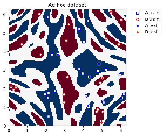
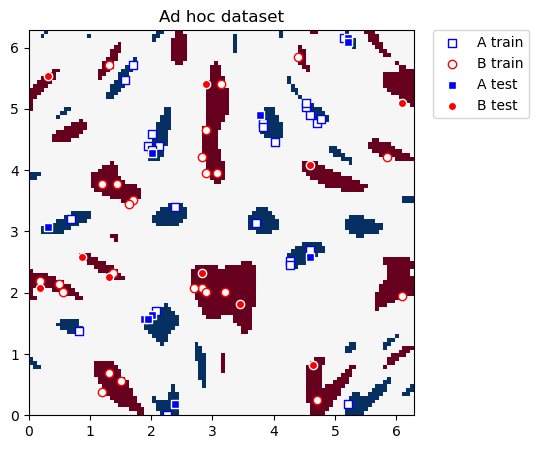
For this example, we will use the ad hoc dataset as described in the reference paper.
We can define the dataset dimension and get our train and test subsets:
[2]:
from qiskit_machine_learning.datasets import ad_hoc_data

adhoc_dimension = 2
train_features, train_labels, test_features, test_labels, adhoc_total = ad_hoc_data(
    training_size=20,
    test_size=5,
    n=adhoc_dimension,
    gap=0.3,
    plot_data=False,
    one_hot=False,
    include_sample_total=True,
)
This dataset is two-dimensional, the two features are represented by the \(x\) and \(y\) coordinates, and it has two class labels: A and B. We can plot it and see what the distribution looks like. We define utility functions to plot the dataset.
[3]:
import matplotlib.pyplot as plt
import numpy as np


def plot_features(ax, features, labels, class_label, marker, face, edge, label):
    # A train plot
    ax.scatter(
        # x coordinate of labels where class is class_label
        features[np.where(labels[:] == class_label), 0],
        # y coordinate of labels where class is class_label
        features[np.where(labels[:] == class_label), 1],
        marker=marker,
        facecolors=face,
        edgecolors=edge,
        label=label,
    )


def plot_dataset(train_features, train_labels, test_features, test_labels, adhoc_total):

    plt.figure(figsize=(5, 5))
    plt.ylim(0, 2 * np.pi)
    plt.xlim(0, 2 * np.pi)
    plt.imshow(
        np.asmatrix(adhoc_total).T,
        interpolation="nearest",
        origin="lower",
        cmap="RdBu",
        extent=[0, 2 * np.pi, 0, 2 * np.pi],
    )

    # A train plot
    plot_features(plt, train_features, train_labels, 0, "s", "w", "b", "A train")

    # B train plot
    plot_features(plt, train_features, train_labels, 1, "o", "w", "r", "B train")

    # A test plot
    plot_features(plt, test_features, test_labels, 0, "s", "b", "w", "A test")

    # B test plot
    plot_features(plt, test_features, test_labels, 1, "o", "r", "w", "B test")

    plt.legend(bbox_to_anchor=(1.05, 1), loc="upper left", borderaxespad=0.0)
    plt.title("Ad hoc dataset")

    plt.show()
Now we actually plot the dataset for classification:
[4]:
plot_dataset(train_features, train_labels, test_features, test_labels, adhoc_total)
2.2. Defining the quantum kernel#
The next step is to create a quantum kernel instance that will help classify this data.
We use the FidelityQuantumKernel class, and pass two input arguments to its constructor:
feature_map: in this case, a two-qubit ZZFeatureMap.fidelity: in this case, the ComputeUncompute fidelity subroutine that leverages the Sampler primitive.
NOTE: If you don’t pass a Sampler or Fidelity instance, then the instances of the reference Sampler and ComputeUncompute classes (found in qiskit.primitives) will be created by default.
[5]:
from qiskit.circuit.library import ZZFeatureMap
from qiskit.primitives import Sampler
from qiskit_algorithms.state_fidelities import ComputeUncompute
from qiskit_machine_learning.kernels import FidelityQuantumKernel

adhoc_feature_map = ZZFeatureMap(feature_dimension=adhoc_dimension, reps=2, entanglement="linear")

sampler = Sampler()

fidelity = ComputeUncompute(sampler=sampler)

adhoc_kernel = FidelityQuantumKernel(fidelity=fidelity, feature_map=adhoc_feature_map)
2.3. Classification with SVC#
The quantum kernel can now be plugged into classical kernel methods, such as the SVC algorithm from scikit-learn. This algorithm allows us to define a custom kernel in two ways:
by providing the kernel as a callable function
by precomputing the kernel matrix
Kernel as a callable function#
We define a SVC model and directly pass the evaluate function of the quantum kernel as a callable. Once the model is created, we train it by calling the fit method on the training dataset and evaluate the model for accuracy with score.
[6]:
from sklearn.svm import SVC

adhoc_svc = SVC(kernel=adhoc_kernel.evaluate)

adhoc_svc.fit(train_features, train_labels)

adhoc_score_callable_function = adhoc_svc.score(test_features, test_labels)

print(f"Callable kernel classification test score: {adhoc_score_callable_function}")
Callable kernel classification test score: 1.0
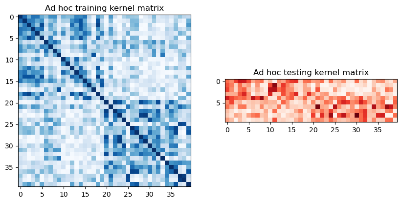
Precomputed kernel matrix#
Instead of passing a function of the quantum kernel as a callable, we can also precompute training and testing kernel matrices before passing them to the scikit-learn SVC algorithm.
To extract the train and test matrices, we can call evaluate on the previously defined kernel and visualize them graphically as follows:
[7]:
adhoc_matrix_train = adhoc_kernel.evaluate(x_vec=train_features)
adhoc_matrix_test = adhoc_kernel.evaluate(x_vec=test_features, y_vec=train_features)

fig, axs = plt.subplots(1, 2, figsize=(10, 5))

axs[0].imshow(
    np.asmatrix(adhoc_matrix_train), interpolation="nearest", origin="upper", cmap="Blues"
)
axs[0].set_title("Ad hoc training kernel matrix")

axs[1].imshow(np.asmatrix(adhoc_matrix_test), interpolation="nearest", origin="upper", cmap="Reds")
axs[1].set_title("Ad hoc testing kernel matrix")

plt.show()
To use these matrices, we set the kernel parameter of a new SVC instance to "precomputed". We train the classifier by calling fit with the training matrix and training dataset. Once the model is trained, we evaluate it using the test matrix on the test dataset.
[8]:
adhoc_svc = SVC(kernel="precomputed")

adhoc_svc.fit(adhoc_matrix_train, train_labels)

adhoc_score_precomputed_kernel = adhoc_svc.score(adhoc_matrix_test, test_labels)

print(f"Precomputed kernel classification test score: {adhoc_score_precomputed_kernel}")
Precomputed kernel classification test score: 1.0
2.4. Classification with QSVC#
QSVC is an alternative training algorithm provided by qiskit-machine-learning for convenience. It is an extension of SVC that takes in a quantum kernel instead of the kernel.evaluate method shown before.
[9]:
from qiskit_machine_learning.algorithms import QSVC

qsvc = QSVC(quantum_kernel=adhoc_kernel)

qsvc.fit(train_features, train_labels)

qsvc_score = qsvc.score(test_features, test_labels)

print(f"QSVC classification test score: {qsvc_score}")
QSVC classification test score: 1.0
2.5. Evaluation of models used for classification#
[10]:
print(f"Classification Model                    | Accuracy Score")
print(f"---------------------------------------------------------")
print(f"SVC using kernel as a callable function | {adhoc_score_callable_function:10.2f}")
print(f"SVC using precomputed kernel matrix     | {adhoc_score_precomputed_kernel:10.2f}")
print(f"QSVC                                    | {qsvc_score:10.2f}")
Classification Model                    | Accuracy Score
---------------------------------------------------------
SVC using kernel as a callable function |       1.00
SVC using precomputed kernel matrix     |       1.00
QSVC                                    |       1.00
As the classification dataset is small, we find that the three models achieve 100% accuracy.
3. Clustering#
The second workflow in this tutorial focuses on a clustering task using qiskit-machine-learning and the spectral clustering algorithm from scikit-learn.
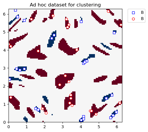
3.1. Defining the dataset#
We will once again use the ad hoc dataset, but now generated with a higher gap of 0.6 (previous example: 0.3) between the two classes.
Note that clustering falls under the category of unsupervised machine learning, so a test dataset is not required.
[11]:
adhoc_dimension = 2
train_features, train_labels, test_features, test_labels, adhoc_total = ad_hoc_data(
    training_size=25,
    test_size=0,
    n=adhoc_dimension,
    gap=0.6,
    plot_data=False,
    one_hot=False,
    include_sample_total=True,
)
We plot the clustering dataset below:
[12]:
plt.figure(figsize=(5, 5))
plt.ylim(0, 2 * np.pi)
plt.xlim(0, 2 * np.pi)
plt.imshow(
    np.asmatrix(adhoc_total).T,
    interpolation="nearest",
    origin="lower",
    cmap="RdBu",
    extent=[0, 2 * np.pi, 0, 2 * np.pi],
)

# A label plot
plot_features(plt, train_features, train_labels, 0, "s", "w", "b", "B")

# B label plot
plot_features(plt, train_features, train_labels, 1, "o", "w", "r", "B")

plt.legend(bbox_to_anchor=(1.05, 1), loc="upper left", borderaxespad=0.0)
plt.title("Ad hoc dataset for clustering")

plt.show()
3.2. Defining the Quantum Kernel#
We use an identical setup as in the classification example. We create another instance of the FidelityQuantumKernel class with a ZZFeatureMap, but you might notice that in this case we do not provide a fidelity instance. This is because the ComputeUncompute method provided in the previous case is instantiated by default when the fidelity instance is not provided explicitly.
[13]:
adhoc_feature_map = ZZFeatureMap(feature_dimension=adhoc_dimension, reps=2, entanglement="linear")

adhoc_kernel = FidelityQuantumKernel(feature_map=adhoc_feature_map)
3.3. Clustering with the Spectral Clustering Model#
The scikit-learn spectral clustering algorithm allows us to define a custom kernel in two ways (just like SVC):
by providing the kernel as a callable function
by precomputing the kernel matrix.
With the current FidelityQuantumKernel class in qiskit-machine-learning, we can only use the latter option, so we precompute the kernel matrix by calling evaluate and visualize it as follows:
[14]:
adhoc_matrix = adhoc_kernel.evaluate(x_vec=train_features)

plt.figure(figsize=(5, 5))
plt.imshow(np.asmatrix(adhoc_matrix), interpolation="nearest", origin="upper", cmap="Greens")
plt.title("Ad hoc clustering kernel matrix")
plt.show()
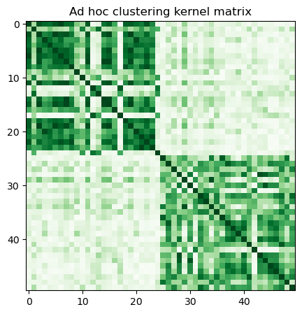
Next, we define a spectral clustering model and fit it using the precomputed kernel. Further, we score the labels using normalized mutual information, since we know the class labels a priori (before hand).
[15]:
from sklearn.cluster import SpectralClustering
from sklearn.metrics import normalized_mutual_info_score

adhoc_spectral = SpectralClustering(2, affinity="precomputed")

cluster_labels = adhoc_spectral.fit_predict(adhoc_matrix)

cluster_score = normalized_mutual_info_score(cluster_labels, train_labels)

print(f"Clustering score: {cluster_score}")
Clustering score: 0.7287008798015754
4. Kernel Principal Component Analysis#
This section focuses on a Principal Component Analysis task using a kernel PCA algorithm. We calculate a kernel matrix using a ZZFeatureMap and show that this approach translates the original features into a new space, where axes are chosen along principal components. In this space the classification task can be performed with a simpler model rather than an SVM.
4.1. Defining the dataset#
We again use the ad hoc dataset with a gap of 0.6 between the two classes. This dataset resembles the dataset we had in the clustering section, the difference is that in this case test_size is not zero.
[16]:
adhoc_dimension = 2
train_features, train_labels, test_features, test_labels, adhoc_total = ad_hoc_data(
    training_size=25,
    test_size=10,
    n=adhoc_dimension,
    gap=0.6,
    plot_data=False,
    one_hot=False,
    include_sample_total=True,
)
We plot the training and test datasets below. Our ultimate goal in this section is to construct new coordinates where the two classes can be linearly separated.
[17]:
plot_dataset(train_features, train_labels, test_features, test_labels, adhoc_total)
4.2. Defining the Quantum Kernel#
We proceed with the same kernel setup as it was in the classification task, namely a ZZFeatureMap circuit as a feature map and an instance of FidelityQuantumKernel.
[18]:
feature_map = ZZFeatureMap(feature_dimension=2, reps=2, entanglement="linear")
qpca_kernel = FidelityQuantumKernel(fidelity=fidelity, feature_map=feature_map)
Then, we evaluate kernel matrices for the training and test features.
[19]:
matrix_train = qpca_kernel.evaluate(x_vec=train_features)
matrix_test = qpca_kernel.evaluate(x_vec=test_features, y_vec=train_features)
4.3. Comparison of Kernel PCA on gaussian and quantum kernel#
In this section we use the KernelPCA implementation from scikit-learn, with the kernel parameter set to "rbf" for a gaussian kernel and "precomputed" for a quantum kernel. The former is very popular in classical machine learning models, whereas the latter allows using a quantum kernel defined as qpca_kernel.
One can observe that the gaussian kernel based Kernel PCA model fails to make the dataset linearly separable, while the quantum kernel succeeds.
While usually PCA is used to reduce the number of features in a dataset, or in other words to reduce dimensionality of a dataset, we don’t do that here. Rather we keep the number of dimensions and employ the kernel PCA, mostly for visualization purposes, to show that classification on the transformed dataset becomes easily tractable by linear methods, like logistic regression. We use this method to separate two classes in the principal component space with a LogisticRegression model from
scikit-learn. As usual we train it by calling the fit method on the training dataset and evaluate the model for accuracy with score.
[20]:
from sklearn.decomposition import KernelPCA

kernel_pca_rbf = KernelPCA(n_components=2, kernel="rbf")
kernel_pca_rbf.fit(train_features)
train_features_rbf = kernel_pca_rbf.transform(train_features)
test_features_rbf = kernel_pca_rbf.transform(test_features)

kernel_pca_q = KernelPCA(n_components=2, kernel="precomputed")
train_features_q = kernel_pca_q.fit_transform(matrix_train)
test_features_q = kernel_pca_q.transform(matrix_test)
Here we train and score a model.
[21]:
from sklearn.linear_model import LogisticRegression

logistic_regression = LogisticRegression()
logistic_regression.fit(train_features_q, train_labels)

logistic_score = logistic_regression.score(test_features_q, test_labels)
print(f"Logistic regression score: {logistic_score}")
Logistic regression score: 0.9
Let’s plot the results. First, we plot the transformed dataset we get with the quantum kernel. On the same plot we also add model results. Then, we plot the transformed dataset we get with the gaussian kernel.
[22]:
fig, (q_ax, rbf_ax) = plt.subplots(1, 2, figsize=(10, 5))


plot_features(q_ax, train_features_q, train_labels, 0, "s", "w", "b", "A train")
plot_features(q_ax, train_features_q, train_labels, 1, "o", "w", "r", "B train")

plot_features(q_ax, test_features_q, test_labels, 0, "s", "b", "w", "A test")
plot_features(q_ax, test_features_q, test_labels, 1, "o", "r", "w", "A test")

q_ax.set_ylabel("Principal component #1")
q_ax.set_xlabel("Principal component #0")
q_ax.set_title("Projection of training and test data\n using KPCA with Quantum Kernel")

# Plotting the linear separation
h = 0.01  # step size in the mesh

# create a mesh to plot in
x_min, x_max = train_features_q[:, 0].min() - 1, train_features_q[:, 0].max() + 1
y_min, y_max = train_features_q[:, 1].min() - 1, train_features_q[:, 1].max() + 1
xx, yy = np.meshgrid(np.arange(x_min, x_max, h), np.arange(y_min, y_max, h))

predictions = logistic_regression.predict(np.c_[xx.ravel(), yy.ravel()])

# Put the result into a color plot
predictions = predictions.reshape(xx.shape)
q_ax.contourf(xx, yy, predictions, cmap=plt.cm.RdBu, alpha=0.2)

plot_features(rbf_ax, train_features_rbf, train_labels, 0, "s", "w", "b", "A train")
plot_features(rbf_ax, train_features_rbf, train_labels, 1, "o", "w", "r", "B train")
plot_features(rbf_ax, test_features_rbf, test_labels, 0, "s", "b", "w", "A test")
plot_features(rbf_ax, test_features_rbf, test_labels, 1, "o", "r", "w", "A test")

rbf_ax.set_ylabel("Principal component #1")
rbf_ax.set_xlabel("Principal component #0")
rbf_ax.set_title("Projection of training data\n using KernelPCA")
plt.show()
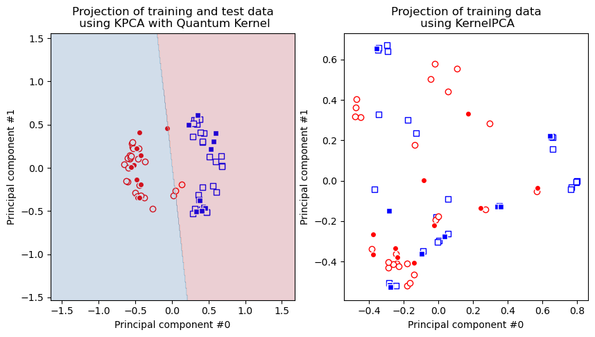
As we can see, the data points on the right figure are not separable, but they are on the left figure, hence in case of quantum kernel we can apply linear models on the transformed dataset and this is why SVM classifier works perfectly well on the ad hoc dataset as we saw in the classification section.
5. Conclusion#
In this tutorial:
We reviewed the fundamentals of quantum kernel learning
We understood how to define quantum kernels as instances of
FidelityQuantumKernelWe learned how to use the
scikit-learnSVCalgorithm with a custom quantum kernel as a callable function vs precomputed quantum kernel matrix for classificationWe learned how to train classifiers with the
QSVCalgorithm fromqiskit-machine-learningWe learned how to use the
scikit-learnSpectralClusteringalgorithms with a precomputed quantum kernel matrix for clusteringWe investigated how to plug in a quantum kernel into
scikit-learn’sKernelPCAalgorithm and transform the ad-hoc dataset into a new one that can be tackled by a linear model.
For further reference, scikit-learn has other algorithms that can use a precomputed kernel matrix, such as:
क्लस्टरिंग ढेर <https://scikit-learn.org/stable/modules/generated/sklearn.cluster.AgglomerativeClustering.html>`__
सहयोग वैक्टर प्रतिगमन <https://scikit-learn.org/stable/modules/generated/sklearn.svm.SVR.html>`__
चोटी प्रतिगमन <https://scikit-learn.org/stable/modules/generated/sklearn.kernel_ridge.KernelRidge.html>`__
[23]:
import qiskit.tools.jupyter

%qiskit_version_table
%qiskit_copyright
Version Information
| Qiskit Software | Version |
|---|---|
qiskit-terra | 0.23.1 |
qiskit-aer | 0.11.2 |
qiskit-ibmq-provider | 0.20.0 |
qiskit | 0.41.0 |
qiskit-machine-learning | 0.5.0 |
| System information | |
| Python version | 3.10.9 |
| Python compiler | GCC 11.2.0 |
| Python build | main, Jan 11 2023 15:21:40 |
| OS | Linux |
| CPUs | 10 |
| Memory (Gb) | 7.394691467285156 |
| Wed Feb 22 10:36:16 2023 CET | |
This code is a part of Qiskit
© Copyright IBM 2017, 2023.
This code is licensed under the Apache License, Version 2.0. You may
obtain a copy of this license in the LICENSE.txt file in the root directory
of this source tree or at http://www.apache.org/licenses/LICENSE-2.0.
Any modifications or derivative works of this code must retain this
copyright notice, and modified files need to carry a notice indicating
that they have been altered from the originals.