Nota

Esta página fue generada a partir de docs/tutorials/09_credit_risk_analysis.ipynb.

Análisis de Riesgo Crediticio

Introducción

Este tutorial muestra cómo se pueden utilizar los algoritmos cuánticos para el análisis de riesgo crediticio. Más precisamente, cómo se puede utilizar la Estimación de Amplitud Cuántica (Quantum Amplitude Estimation, QAE) para estimar medidas de riesgo con una aceleración cuadrática sobre la simulación clásica de Monte Carlo. El tutorial se basa en los siguientes artículos:

• Quantum Risk Analysis. Stefan Woerner, Daniel J. Egger. [Woerner2019]

• Credit Risk Analysis using Quantum Computers. Egger et al. (2019) [Egger2019]

Se puede encontrar una introducción general a QAE en el siguiente documento:

• Quantum Amplitude Amplification and Estimation. Gilles Brassard et al.

La estructura del tutorial es la siguiente:

1. Definición del Problema

2. Modelo de Incertidumbre

3. Pérdida Esperada

4. Función de Distribución Acumulativa

5. Valor en Riesgo

6. Valor en Riesgo Condicional

import numpy as np
import matplotlib.pyplot as plt

from qiskit import QuantumRegister, QuantumCircuit
from qiskit.circuit.library import IntegerComparator
from qiskit_algorithms import IterativeAmplitudeEstimation, EstimationProblem
from qiskit_aer.primitives import Sampler

Definición del Problema

En este tutorial queremos analizar el riesgo crediticio de una cartera de \(K\) activos. La probabilidad predeterminada de cada activo \(k\) sigue un modelo de Independencia Condicional Gaussiana, es decir, dado un valor \(z\) muestreado a partir de una variable aleatoria latente \(Z\) siguiendo una distribución normal estándar, la probabilidad predeterminada del activo \(k\) está dada por

\[p_k(z) = F\left( \frac{F^{-1}(p_k^0) - \sqrt{\rho_k}z}{\sqrt{1 - \rho_k}} \right)\]

donde \(F\) denota la función de distribución acumulativa de \(Z\), \(p_k^0\) es la probabilidad predeterminada del activo \(k\) para \(z=0\) y \(\rho_k\) es la sensibilidad de la probabilidad predeterminada del activo \(k\) con respecto a \(Z\). Por lo tanto, dada una realización concreta de \(Z\), los eventos individuales predeterminados se suponen independientes entre sí.

Estamos interesados en analizar las medidas de riesgo de la pérdida total

\[L = \sum_{k=1}^K \lambda_k X_k(Z)\]

donde \(\lambda_k\) denota la pérdida dado el incumplimiento del activo \(k\), y dada \(Z\), \(X_k(Z)\) denota una variable de Bernoulli que representa el evento predeterminado del activo \(k\). Más precisamente, estamos interesados en el valor esperado \(\mathbb{E}[L]\), el valor en riesgo (Value at Risk, VaR) de \(L\) y el Valor en Riesgo Condicional de \(L\) (también llamado Déficit Esperado). Donde VaR y CVaR se definen como

\[\text{VaR}_{\alpha}(L) = \inf \{ x \mid \mathbb{P}[L <= x] \geq 1 - \alpha \}\]

con nivel de confianza \(\alpha \in [0, 1]\), y

\[\text{CVaR}_{\alpha}(L) = \mathbb{E}[ L \mid L \geq \text{VaR}_{\alpha}(L) ].\]

Para obtener más detalles sobre el modelo considerado, consulta, por ejemplo, Regulatory Capital Modeling for Credit Risk. Marek Rutkowski, Silvio Tarca

El problema está definido por los siguientes parámetros:

• número de qubits utilizados para representar \(Z\), indicado por \(n_z\)

• valor de truncamiento para \(Z\), denotado por \(z_{\text{max}}\), es decir, se supone que Z toma \(2^{n_z}\) valores equidistantes en \(\{-z_{max}, ..., +z_{max}\}\)

• las probabilidades base por defecto para cada activo \(p_0^k \in (0, 1)\), \(k=1, ..., K\)

• sensibilidades de las probabilidades predeterminadas con respecto a \(Z\), indicadas por \(\rho_k \in [0, 1)\)

• pérdida dado el incumplimiento para el activo \(k\), indicada por \(\lambda_k\)

• nivel de confianza para VaR / CVaR \(\alpha \in [0, 1]\).

# set problem parameters
n_z = 2
z_max = 2
z_values = np.linspace(-z_max, z_max, 2**n_z)
p_zeros = [0.15, 0.25]
rhos = [0.1, 0.05]
lgd = [1, 2]
K = len(p_zeros)
alpha = 0.05

Modelo de Incertidumbre

Ahora construimos un circuito que carga el modelo de incertidumbre. Esto se puede lograr creando un estado cuántico en un registro de \(n_z\) qubits que represente a \(Z\) siguiendo una distribución normal estándar. Este estado luego se usa para controlar rotaciones Y de un solo qubit sobre un segundo registro de qubit de \(K\) qubits, donde el estado \(|1\rangle\) del qubit \(k\) representa el evento predeterminado del activo \(k\). El estado cuántico resultante se puede escribir como

\[ |\Psi\rangle = \sum_{i=0}^{2^{n_z}-1} \sqrt{p_z^i} |z_i \rangle \bigotimes_{k=1}^K \left( \sqrt{1 - p_k(z_i)}|0\rangle + \sqrt{p_k(z_i)}|1\rangle\right),\]

donde denotamos por \(z_i\) el \(i\)-ésimo valor de \(Z\) truncado y discretizado [Egger2019].

from qiskit_finance.circuit.library import GaussianConditionalIndependenceModel as GCI

u = GCI(n_z, z_max, p_zeros, rhos)

u.draw()

     ┌───────┐
q_0: ┤0      ├
     │       │
q_1: ┤1      ├
     │  P(X) │
q_2: ┤2      ├
     │       │
q_3: ┤3      ├
     └───────┘

Ahora usamos el simulador para validar el circuito que construye \(|\Psi\rangle\) y calculamos los valores exactos correspondientes para

• pérdida esperada \(\mathbb{E}[L]\)

• PDF y CDF de \(L\)

• valor en riesgo \(VaR(L)\) y probabilidad correspondiente

• valor en riesgo condicional \(CVaR(L)\)

u_measure = u.measure_all(inplace=False)
sampler = Sampler()
job = sampler.run(u_measure)
binary_probabilities = job.result().quasi_dists[0].binary_probabilities()

# analyze uncertainty circuit and determine exact solutions
p_z = np.zeros(2**n_z)
p_default = np.zeros(K)
values = []
probabilities = []
num_qubits = u.num_qubits

for i, prob in binary_probabilities.items():
    # extract value of Z and corresponding probability
    i_normal = int(i[-n_z:], 2)
    p_z[i_normal] += prob

    # determine overall default probability for k
    loss = 0
    for k in range(K):
        if i[K - k - 1] == "1":
            p_default[k] += prob
            loss += lgd[k]

    values += [loss]
    probabilities += [prob]


values = np.array(values)
probabilities = np.array(probabilities)

expected_loss = np.dot(values, probabilities)
losses = np.sort(np.unique(values))
pdf = np.zeros(len(losses))
for i, v in enumerate(losses):
    pdf[i] += sum(probabilities[values == v])
cdf = np.cumsum(pdf)

i_var = np.argmax(cdf >= 1 - alpha)
exact_var = losses[i_var]
exact_cvar = np.dot(pdf[(i_var + 1) :], losses[(i_var + 1) :]) / sum(pdf[(i_var + 1) :])

print("Expected Loss E[L]:                %.4f" % expected_loss)
print("Value at Risk VaR[L]:              %.4f" % exact_var)
print("P[L <= VaR[L]]:                    %.4f" % cdf[exact_var])
print("Conditional Value at Risk CVaR[L]: %.4f" % exact_cvar)

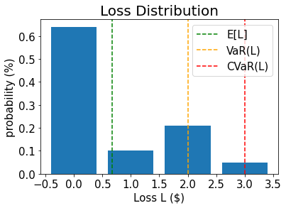
Expected Loss E[L]:                0.6641
Value at Risk VaR[L]:              2.0000
P[L <= VaR[L]]:                    0.9521
Conditional Value at Risk CVaR[L]: 3.0000

# plot loss PDF, expected loss, var, and cvar
plt.bar(losses, pdf)
plt.axvline(expected_loss, color="green", linestyle="--", label="E[L]")
plt.axvline(exact_var, color="orange", linestyle="--", label="VaR(L)")
plt.axvline(exact_cvar, color="red", linestyle="--", label="CVaR(L)")
plt.legend(fontsize=15)
plt.xlabel("Loss L ($)", size=15)
plt.ylabel("probability (%)", size=15)
plt.title("Loss Distribution", size=20)
plt.xticks(size=15)
plt.yticks(size=15)
plt.show()

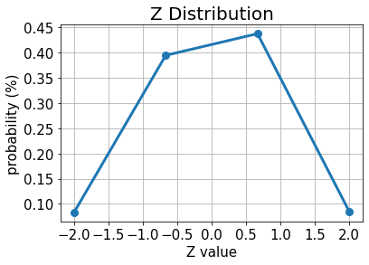
# plot results for Z
plt.plot(z_values, p_z, "o-", linewidth=3, markersize=8)
plt.grid()
plt.xlabel("Z value", size=15)
plt.ylabel("probability (%)", size=15)
plt.title("Z Distribution", size=20)
plt.xticks(size=15)
plt.yticks(size=15)
plt.show()

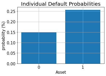
# plot results for default probabilities
plt.bar(range(K), p_default)
plt.xlabel("Asset", size=15)
plt.ylabel("probability (%)", size=15)
plt.title("Individual Default Probabilities", size=20)
plt.xticks(range(K), size=15)
plt.yticks(size=15)
plt.grid()
plt.show()

Pérdida Esperada

Para estimar la pérdida esperada, primero aplicamos un operador de suma ponderada para sumar las pérdidas individuales a la pérdida total:

\[\mathcal{S}: |x_1, ..., x_K \rangle_K |0\rangle_{n_S} \mapsto |x_1, ..., x_K \rangle_K |\lambda_1x_1 + ... + \lambda_K x_K\rangle_{n_S}.\]

El número requerido de qubits para representar el resultado está dado por

\[n_s = \lfloor \log_2( \lambda_1 + ... + \lambda_K ) \rfloor + 1.\]

Una vez que tenemos la distribución de pérdida total en un registro cuántico, podemos utilizar las técnicas descritas en [Woerner2019] para asignar una pérdida total \(L \in \{0, ..., 2^{n_s}-1\}\) a la amplitud de un qubit objetivo por un operador

\[ | L \rangle_{n_s}|0\rangle \mapsto | L \rangle_{n_s} \left( \sqrt{1 - L/(2^{n_s}-1)}|0\rangle + \sqrt{L/(2^{n_s}-1)}|1\rangle \right),\]

que permite ejecutar la estimación de amplitud para evaluar la pérdida esperada.

# add Z qubits with weight/loss 0
from qiskit.circuit.library import WeightedAdder

agg = WeightedAdder(n_z + K, [0] * n_z + lgd)

from qiskit.circuit.library import LinearAmplitudeFunction

# define linear objective function
breakpoints = [0]
slopes = [1]
offsets = [0]
f_min = 0
f_max = sum(lgd)
c_approx = 0.25

objective = LinearAmplitudeFunction(
    agg.num_sum_qubits,
    slope=slopes,
    offset=offsets,
    # max value that can be reached by the qubit register (will not always be reached)
    domain=(0, 2**agg.num_sum_qubits - 1),
    image=(f_min, f_max),
    rescaling_factor=c_approx,
    breakpoints=breakpoints,
)

Crear el circuito de preparación de estado:

# define the registers for convenience and readability
qr_state = QuantumRegister(u.num_qubits, "state")
qr_sum = QuantumRegister(agg.num_sum_qubits, "sum")
qr_carry = QuantumRegister(agg.num_carry_qubits, "carry")
qr_obj = QuantumRegister(1, "objective")

# define the circuit
state_preparation = QuantumCircuit(qr_state, qr_obj, qr_sum, qr_carry, name="A")

# load the random variable
state_preparation.append(u.to_gate(), qr_state)

# aggregate
state_preparation.append(agg.to_gate(), qr_state[:] + qr_sum[:] + qr_carry[:])

# linear objective function
state_preparation.append(objective.to_gate(), qr_sum[:] + qr_obj[:])

# uncompute aggregation
state_preparation.append(agg.to_gate().inverse(), qr_state[:] + qr_sum[:] + qr_carry[:])

# draw the circuit
state_preparation.draw()

           ┌───────┐┌────────┐      ┌───────────┐
  state_0: ┤0      ├┤0       ├──────┤0          ├
           │       ││        │      │           │
  state_1: ┤1      ├┤1       ├──────┤1          ├
           │  P(X) ││        │      │           │
  state_2: ┤2      ├┤2       ├──────┤2          ├
           │       ││        │      │           │
  state_3: ┤3      ├┤3       ├──────┤3          ├
           └───────┘│  adder │┌────┐│  adder_dg │
objective: ─────────┤        ├┤2   ├┤           ├
                    │        ││    ││           │
    sum_0: ─────────┤4       ├┤0 F ├┤4          ├
                    │        ││    ││           │
    sum_1: ─────────┤5       ├┤1   ├┤5          ├
                    │        │└────┘│           │
    carry: ─────────┤6       ├──────┤6          ├
                    └────────┘      └───────────┘

Antes de usar QAE para estimar la pérdida esperada, validamos el circuito cuántico que representa la función objetivo simplemente simulándolo directamente y analizando la probabilidad de que el qubit objetivo esté en el estado \(|1\rangle\), es decir, el valor que QAE eventualmente aproximará.

state_preparation_measure = state_preparation.measure_all(inplace=False)
sampler = Sampler()
job = sampler.run(state_preparation_measure)
binary_probabilities = job.result().quasi_dists[0].binary_probabilities()

# evaluate the result
value = 0
for i, prob in binary_probabilities.items():
    if prob > 1e-6 and i[-(len(qr_state) + 1) :][0] == "1":
        value += prob

print("Exact Expected Loss:   %.4f" % expected_loss)
print("Exact Operator Value:  %.4f" % value)
print("Mapped Operator value: %.4f" % objective.post_processing(value))

Exact Expected Loss:   0.6641
Exact Operator Value:  0.3789
Mapped Operator value: 0.5749

A continuación ejecutamos QAE para estimar la pérdida esperada con una aceleración cuadrática sobre la simulación clásica de Monte Carlo.

# set target precision and confidence level
epsilon = 0.01
alpha = 0.05

problem = EstimationProblem(
    state_preparation=state_preparation,
    objective_qubits=[len(qr_state)],
    post_processing=objective.post_processing,
)
# construct amplitude estimation
ae = IterativeAmplitudeEstimation(
    epsilon_target=epsilon, alpha=alpha, sampler=Sampler(run_options={"shots": 100, "seed": 75})
)
result = ae.estimate(problem)

# print results
conf_int = np.array(result.confidence_interval_processed)
print("Exact value:    \t%.4f" % expected_loss)
print("Estimated value:\t%.4f" % result.estimation_processed)
print("Confidence interval: \t[%.4f, %.4f]" % tuple(conf_int))

Exact value:            0.6641
Estimated value:        0.6863
Confidence interval:    [0.6175, 0.7552]

Función de Distribución Acumulativa

En lugar de la pérdida esperada (que también podría estimarse de manera eficiente utilizando técnicas clásicas), ahora estimamos la función de distribución acumulada (CDF) de la pérdida. Clásicamente, esto implica evaluar todas las posibles combinaciones de activos en incumplimiento o muchas muestras clásicas en una simulación Monte Carlo. Los algoritmos basados en QAE tienen el potencial de acelerar significativamente este análisis en el futuro.

Para estimar el CDF, es decir, la probabilidad \(\mathbb{P}[L \leq x]\), aplicamos nuevamente \(\mathcal{S}\) para calcular la pérdida total, y luego aplicamos un comparador que para un valor dado \(x\) actúa como

\[\begin{split} \mathcal{C}: |L\rangle_n|0> \mapsto \begin{cases} |L\rangle_n|1> & \text{si}\quad L \leq x \\ |L\rangle_n|0> & \text{si}\quad L > x. \end{cases}\end{split}\]

El estado cuántico resultante se puede escribir como

\[ \sum_{L = 0}^{x} \sqrt{p_{L}}|L\rangle_{n_s}|1\rangle + \sum_{L = x+1}^{2^{n_s}-1} \sqrt{p_{L}}|L\rangle_{n_s}|0\rangle,\]

donde asumimos directamente los valores de pérdida sumados y las probabilidades correspondientes en lugar de presentar los detalles del modelo de incertidumbre.

La CDF(\(x\)) es igual a la probabilidad de medir \(|1\rangle\) en el qubit objetivo y se puede utilizar directamente QAE para estimarlo.

# set x value to estimate the CDF
x_eval = 2

comparator = IntegerComparator(agg.num_sum_qubits, x_eval + 1, geq=False)
comparator.draw()

         ┌──────┐
state_0: ┤0     ├
         │      │
state_1: ┤1     ├
         │  cmp │
compare: ┤2     ├
         │      │
    a15: ┤3     ├
         └──────┘

def get_cdf_circuit(x_eval):
    # define the registers for convenience and readability
    qr_state = QuantumRegister(u.num_qubits, "state")
    qr_sum = QuantumRegister(agg.num_sum_qubits, "sum")
    qr_carry = QuantumRegister(agg.num_carry_qubits, "carry")
    qr_obj = QuantumRegister(1, "objective")
    qr_compare = QuantumRegister(1, "compare")

    # define the circuit
    state_preparation = QuantumCircuit(qr_state, qr_obj, qr_sum, qr_carry, name="A")

    # load the random variable
    state_preparation.append(u, qr_state)

    # aggregate
    state_preparation.append(agg, qr_state[:] + qr_sum[:] + qr_carry[:])

    # comparator objective function
    comparator = IntegerComparator(agg.num_sum_qubits, x_eval + 1, geq=False)
    state_preparation.append(comparator, qr_sum[:] + qr_obj[:] + qr_carry[:])

    # uncompute aggregation
    state_preparation.append(agg.inverse(), qr_state[:] + qr_sum[:] + qr_carry[:])

    return state_preparation


state_preparation = get_cdf_circuit(x_eval)

Nuevamente, primero utilizamos la simulación cuántica para validar el circuito cuántico.

state_preparation.draw()

           ┌───────┐┌────────┐        ┌───────────┐
  state_0: ┤0      ├┤0       ├────────┤0          ├
           │       ││        │        │           │
  state_1: ┤1      ├┤1       ├────────┤1          ├
           │  P(X) ││        │        │           │
  state_2: ┤2      ├┤2       ├────────┤2          ├
           │       ││        │        │           │
  state_3: ┤3      ├┤3       ├────────┤3          ├
           └───────┘│  adder │┌──────┐│  adder_dg │
objective: ─────────┤        ├┤2     ├┤           ├
                    │        ││      ││           │
    sum_0: ─────────┤4       ├┤0     ├┤4          ├
                    │        ││  cmp ││           │
    sum_1: ─────────┤5       ├┤1     ├┤5          ├
                    │        ││      ││           │
    carry: ─────────┤6       ├┤3     ├┤6          ├
                    └────────┘└──────┘└───────────┘

state_preparation_measure = state_preparation.measure_all(inplace=False)
sampler = Sampler()
job = sampler.run(state_preparation_measure)
binary_probabilities = job.result().quasi_dists[0].binary_probabilities()

# evaluate the result
var_prob = 0
for i, prob in binary_probabilities.items():
    if prob > 1e-6 and i[-(len(qr_state) + 1) :][0] == "1":
        var_prob += prob

print("Operator CDF(%s)" % x_eval + " = %.4f" % var_prob)
print("Exact    CDF(%s)" % x_eval + " = %.4f" % cdf[x_eval])

Operator CDF(2) = 0.9551
Exact    CDF(2) = 0.9521

A continuación ejecutamos QAE para estimar la CDF para un \(x\) dado.

# set target precision and confidence level
epsilon = 0.01
alpha = 0.05

problem = EstimationProblem(state_preparation=state_preparation, objective_qubits=[len(qr_state)])
# construct amplitude estimation
ae_cdf = IterativeAmplitudeEstimation(
    epsilon_target=epsilon, alpha=alpha, sampler=Sampler(run_options={"shots": 100, "seed": 75})
)
result_cdf = ae_cdf.estimate(problem)

# print results
conf_int = np.array(result_cdf.confidence_interval)
print("Exact value:    \t%.4f" % cdf[x_eval])
print("Estimated value:\t%.4f" % result_cdf.estimation)
print("Confidence interval: \t[%.4f, %.4f]" % tuple(conf_int))

Exact value:            0.9521
Estimated value:        0.9590
Confidence interval:    [0.9577, 0.9603]

Valor en Riesgo

A continuación utilizamos una búsqueda de bisección y QAE para evaluar eficientemente la CDF para estimar el valor en riesgo.

def run_ae_for_cdf(x_eval, epsilon=0.01, alpha=0.05):

    # construct amplitude estimation
    state_preparation = get_cdf_circuit(x_eval)
    problem = EstimationProblem(
        state_preparation=state_preparation, objective_qubits=[len(qr_state)]
    )
    ae_var = IterativeAmplitudeEstimation(
        epsilon_target=epsilon, alpha=alpha, sampler=Sampler(run_options={"shots": 100, "seed": 75})
    )
    result_var = ae_var.estimate(problem)

    return result_var.estimation

def bisection_search(
    objective, target_value, low_level, high_level, low_value=None, high_value=None
):
    """
    Determines the smallest level such that the objective value is still larger than the target
    :param objective: objective function
    :param target: target value
    :param low_level: lowest level to be considered
    :param high_level: highest level to be considered
    :param low_value: value of lowest level (will be evaluated if set to None)
    :param high_value: value of highest level (will be evaluated if set to None)
    :return: dictionary with level, value, num_eval
    """

    # check whether low and high values are given and evaluated them otherwise
    print("--------------------------------------------------------------------")
    print("start bisection search for target value %.3f" % target_value)
    print("--------------------------------------------------------------------")
    num_eval = 0
    if low_value is None:
        low_value = objective(low_level)
        num_eval += 1
    if high_value is None:
        high_value = objective(high_level)
        num_eval += 1

    # check if low_value already satisfies the condition
    if low_value > target_value:
        return {
            "level": low_level,
            "value": low_value,
            "num_eval": num_eval,
            "comment": "returned low value",
        }
    elif low_value == target_value:
        return {"level": low_level, "value": low_value, "num_eval": num_eval, "comment": "success"}

    # check if high_value is above target
    if high_value < target_value:
        return {
            "level": high_level,
            "value": high_value,
            "num_eval": num_eval,
            "comment": "returned low value",
        }
    elif high_value == target_value:
        return {
            "level": high_level,
            "value": high_value,
            "num_eval": num_eval,
            "comment": "success",
        }

    # perform bisection search until
    print("low_level    low_value    level    value    high_level    high_value")
    print("--------------------------------------------------------------------")
    while high_level - low_level > 1:

        level = int(np.round((high_level + low_level) / 2.0))
        num_eval += 1
        value = objective(level)

        print(
            "%2d           %.3f        %2d       %.3f    %2d            %.3f"
            % (low_level, low_value, level, value, high_level, high_value)
        )

        if value >= target_value:
            high_level = level
            high_value = value
        else:
            low_level = level
            low_value = value

    # return high value after bisection search
    print("--------------------------------------------------------------------")
    print("finished bisection search")
    print("--------------------------------------------------------------------")
    return {"level": high_level, "value": high_value, "num_eval": num_eval, "comment": "success"}

# run bisection search to determine VaR
objective = lambda x: run_ae_for_cdf(x)
bisection_result = bisection_search(
    objective, 1 - alpha, min(losses) - 1, max(losses), low_value=0, high_value=1
)
var = bisection_result["level"]

--------------------------------------------------------------------
start bisection search for target value 0.950
--------------------------------------------------------------------
low_level    low_value    level    value    high_level    high_value
--------------------------------------------------------------------
-1           0.000         1       0.752     3            1.000
 1           0.752         2       0.959     3            1.000
--------------------------------------------------------------------
finished bisection search
--------------------------------------------------------------------

print("Estimated Value at Risk: %2d" % var)
print("Exact Value at Risk:     %2d" % exact_var)
print("Estimated Probability:    %.3f" % bisection_result["value"])
print("Exact Probability:        %.3f" % cdf[exact_var])

Estimated Value at Risk:  2
Exact Value at Risk:      2
Estimated Probability:    0.959
Exact Probability:        0.952

Valor en Riesgo Condicional

Por último, calculamos el CVaR, es decir, el valor esperado de la pérdida condicional a que sea mayor o igual al VaR. Para hacer eso, evaluamos una función objetivo lineal por partes \(f(L)\), dependiente de la pérdida total \(L\), que está dada por

\[\begin{split}f(L) = \begin{cases} 0 & \text{si}\quad L \leq VaR \\ L & \text{si}\quad L > VaR. \end{cases}\end{split}\]

Para normalizar, tenemos que dividir el valor esperado resultante entre la probabilidad de VaR, es decir, \(\mathbb{P}[L \leq VaR]\).

# define linear objective
breakpoints = [0, var]
slopes = [0, 1]
offsets = [0, 0]  # subtract VaR and add it later to the estimate
f_min = 0
f_max = 3 - var
c_approx = 0.25

cvar_objective = LinearAmplitudeFunction(
    agg.num_sum_qubits,
    slopes,
    offsets,
    domain=(0, 2**agg.num_sum_qubits - 1),
    image=(f_min, f_max),
    rescaling_factor=c_approx,
    breakpoints=breakpoints,
)

cvar_objective.draw()

        ┌────┐
q158_0: ┤0   ├
        │    │
q158_1: ┤1   ├
        │    │
  q159: ┤2 F ├
        │    │
 a83_0: ┤3   ├
        │    │
 a83_1: ┤4   ├
        └────┘

# define the registers for convenience and readability
qr_state = QuantumRegister(u.num_qubits, "state")
qr_sum = QuantumRegister(agg.num_sum_qubits, "sum")
qr_carry = QuantumRegister(agg.num_carry_qubits, "carry")
qr_obj = QuantumRegister(1, "objective")
qr_work = QuantumRegister(cvar_objective.num_ancillas - len(qr_carry), "work")

# define the circuit
state_preparation = QuantumCircuit(qr_state, qr_obj, qr_sum, qr_carry, qr_work, name="A")

# load the random variable
state_preparation.append(u, qr_state)

# aggregate
state_preparation.append(agg, qr_state[:] + qr_sum[:] + qr_carry[:])

# linear objective function
state_preparation.append(cvar_objective, qr_sum[:] + qr_obj[:] + qr_carry[:] + qr_work[:])

# uncompute aggregation
state_preparation.append(agg.inverse(), qr_state[:] + qr_sum[:] + qr_carry[:])

<qiskit.circuit.instructionset.InstructionSet at 0x7fdfa88db7f0>

Nuevamente, primero utilizamos la simulación cuántica para validar el circuito cuántico.

state_preparation_measure = state_preparation.measure_all(inplace=False)
sampler = Sampler()
job = sampler.run(state_preparation_measure)
binary_probabilities = job.result().quasi_dists[0].binary_probabilities()

# evaluate the result
value = 0
for i, prob in binary_probabilities.items():
    if prob > 1e-6 and i[-(len(qr_state) + 1)] == "1":
        value += prob

# normalize and add VaR to estimate
value = cvar_objective.post_processing(value)
d = 1.0 - bisection_result["value"]
v = value / d if d != 0 else 0
normalized_value = v + var
print("Estimated CVaR: %.4f" % normalized_value)
print("Exact CVaR:     %.4f" % exact_cvar)

Estimated CVaR: 3.5799
Exact CVaR:     3.0000

A continuación ejecutamos QAE para estimar el CVaR.

# set target precision and confidence level
epsilon = 0.01
alpha = 0.05

problem = EstimationProblem(
    state_preparation=state_preparation,
    objective_qubits=[len(qr_state)],
    post_processing=cvar_objective.post_processing,
)
# construct amplitude estimation
ae_cvar = IterativeAmplitudeEstimation(
    epsilon_target=epsilon, alpha=alpha, sampler=Sampler(run_options={"shots": 100, "seed": 75})
)
result_cvar = ae_cvar.estimate(problem)

# print results
d = 1.0 - bisection_result["value"]
v = result_cvar.estimation_processed / d if d != 0 else 0
print("Exact CVaR:    \t%.4f" % exact_cvar)
print("Estimated CVaR:\t%.4f" % (v + var))

Exact CVaR:     3.0000
Estimated CVaR: 3.3316

import qiskit.tools.jupyter

%qiskit_version_table
%qiskit_copyright

Version Information

Software	Version
qiskit	None
qiskit-terra	0.45.0.dev0+c626be7
qiskit_ibm_provider	0.6.1
qiskit_aer	0.12.0
qiskit_algorithms	0.2.0
qiskit_finance	0.4.0
System information
Python version	3.9.7
Python compiler	GCC 7.5.0
Python build	default, Sep 16 2021 13:09:58
OS	Linux
CPUs	2
Memory (Gb)	5.778430938720703
Fri Aug 18 16:24:38 2023 EDT

This code is a part of Qiskit

© Copyright IBM 2017, 2023.

This code is licensed under the Apache License, Version 2.0. You may
obtain a copy of this license in the LICENSE.txt file in the root directory
of this source tree or at http://www.apache.org/licenses/LICENSE-2.0.

Any modifications or derivative works of this code must retain this
copyright notice, and modified files need to carry a notice indicating
that they have been altered from the originals.