Nota
Esta página fue generada a partir de docs/tutorials/05_bull_spread_pricing.ipynb.
Fijación de Precios de Márgenes Alcistas#
Introducción#
Supón un margen alcista con precios de ejercicio \(K_1 < K_2\) y un activo subyacente cuyo precio al contado al vencimiento \(S_T\) sigue una distribución aleatoria dada. La función de rendimiento correspondiente se define como:
A continuación, se utiliza un algoritmo cuántico basado en la estimación de amplitud para estimar el rendimiento esperado, es decir, el precio justo antes del descuento, para la opción:
así como la correspondiente \(\Delta\), es decir, el derivado del precio de la opción con respecto al precio al contado, definido como:
La aproximación de la función objetivo y una introducción general a la fijación de precios de opciones y el análisis de riesgos en computadoras cuánticas se dan en los siguientes artículos:
[1]:
import matplotlib.pyplot as plt

%matplotlib inline
import numpy as np

from qiskit_algorithms import IterativeAmplitudeEstimation, EstimationProblem
from qiskit.circuit.library import LinearAmplitudeFunction
from qiskit_aer.primitives import Sampler
from qiskit_finance.circuit.library import LogNormalDistribution
Modelo de Incertidumbre#
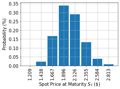
Construimos un circuito para cargar una distribución aleatoria logarítmica normal en un estado cuántico. La distribución se trunca a un intervalo dado \([\text{low}, \text{high}]\) y discretiza usando una cuadrícula con \(2^n\) puntos, donde \(n\) denota el número de qubits utilizados. El operador unitario correspondiente al circuito implementa lo siguiente:
donde \(p_i\) denota las probabilidades correspondientes a la distribución truncada y discretizada y donde \(i\) se asigna al intervalo correcto usando el mapa afín:
[2]:
# number of qubits to represent the uncertainty
num_uncertainty_qubits = 3

# parameters for considered random distribution
S = 2.0  # initial spot price
vol = 0.4  # volatility of 40%
r = 0.05  # annual interest rate of 4%
T = 40 / 365  # 40 days to maturity

# resulting parameters for log-normal distribution
mu = (r - 0.5 * vol**2) * T + np.log(S)
sigma = vol * np.sqrt(T)
mean = np.exp(mu + sigma**2 / 2)
variance = (np.exp(sigma**2) - 1) * np.exp(2 * mu + sigma**2)
stddev = np.sqrt(variance)

# lowest and highest value considered for the spot price; in between, an equidistant discretization is considered.
low = np.maximum(0, mean - 3 * stddev)
high = mean + 3 * stddev

# construct circuit for uncertainty model
uncertainty_model = LogNormalDistribution(
    num_uncertainty_qubits, mu=mu, sigma=sigma**2, bounds=(low, high)
)
[3]:
# plot probability distribution
x = uncertainty_model.values
y = uncertainty_model.probabilities
plt.bar(x, y, width=0.2)
plt.xticks(x, size=15, rotation=90)
plt.yticks(size=15)
plt.grid()
plt.xlabel("Spot Price at Maturity $S_T$ (\$)", size=15)
plt.ylabel("Probability ($\%$)", size=15)
plt.show()
Función de Rendimiento#
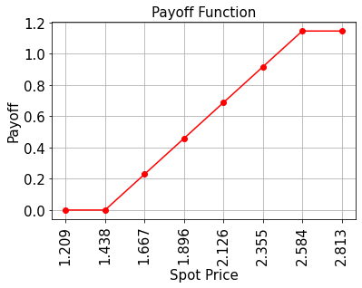
La función de rendimiento es igual a cero siempre que el precio al contado al vencimiento \(S_T\) sea menor que el precio de ejercicio \(K_1\), luego aumenta linealmente y está delimitado por \(K_2\). La implementación usa dos comparadores, que cambian un qubit ancilla cada uno de \(\big|0\rangle\) a \(\big|1\rangle\) si \(S_T \geq K_1\) y \(S_T \leq K_2\), y estas ancillas se utilizan para controlar la parte lineal de la función de rendimiento.
La parte lineal en sí es entonces aproximada de la siguiente manera. Explotamos el hecho de que \(\sin^2(y + \pi/4) \approx y + 1/2\) para pequeños \(|y|\). Por lo tanto, para un factor de reescalado de aproximación dado \(c_\text{approx} \in [0, 1]\) y \(x \in [0, 1]\) consideramos
para pequeños \(c_\text{approx}\).
Podemos construir fácilmente un operador que actúe como
utilizando rotaciones Y controladas.
Finalmente, nos interesa la probabilidad de medir \(\big|1\rangle\) en el último qubit, que corresponde a \(\sin^2(a*x+b)\). Junto con la aproximación anterior, esto permite aproximar los valores de interés. Cuanto más pequeño elijamos \(c_\text{approx}\), mejor será la aproximación. Sin embargo, dado que estamos estimando una propiedad escalada por \(c_\text{approx}\), el número de qubits de evaluación \(m\) debe ajustarse en consecuencia.
Para más detalles sobre la aproximación, nos referimos a: Quantum Risk Analysis. Woerner, Egger. 2018.
[4]:
# set the strike price (should be within the low and the high value of the uncertainty)
strike_price_1 = 1.438
strike_price_2 = 2.584

# set the approximation scaling for the payoff function
rescaling_factor = 0.25

# setup piecewise linear objective fcuntion
breakpoints = [low, strike_price_1, strike_price_2]
slopes = [0, 1, 0]
offsets = [0, 0, strike_price_2 - strike_price_1]
f_min = 0
f_max = strike_price_2 - strike_price_1
bull_spread_objective = LinearAmplitudeFunction(
    num_uncertainty_qubits,
    slopes,
    offsets,
    domain=(low, high),
    image=(f_min, f_max),
    breakpoints=breakpoints,
    rescaling_factor=rescaling_factor,
)

# construct A operator for QAE for the payoff function by
# composing the uncertainty model and the objective
bull_spread = bull_spread_objective.compose(uncertainty_model, front=True)
[5]:
# plot exact payoff function (evaluated on the grid of the uncertainty model)
x = uncertainty_model.values
y = np.minimum(np.maximum(0, x - strike_price_1), strike_price_2 - strike_price_1)
plt.plot(x, y, "ro-")
plt.grid()
plt.title("Payoff Function", size=15)
plt.xlabel("Spot Price", size=15)
plt.ylabel("Payoff", size=15)
plt.xticks(x, size=15, rotation=90)
plt.yticks(size=15)
plt.show()
[6]:
# evaluate exact expected value (normalized to the [0, 1] interval)
exact_value = np.dot(uncertainty_model.probabilities, y)
exact_delta = sum(
    uncertainty_model.probabilities[np.logical_and(x >= strike_price_1, x <= strike_price_2)]
)
print("exact expected value:\t%.4f" % exact_value)
print("exact delta value:   \t%.4f" % exact_delta)
exact expected value:   0.5695
exact delta value:      0.9291
Evaluar el Rendimiento Esperado#
[7]:
# set target precision and confidence level
epsilon = 0.01
alpha = 0.05

problem = EstimationProblem(
    state_preparation=bull_spread,
    objective_qubits=[num_uncertainty_qubits],
    post_processing=bull_spread_objective.post_processing,
)
# construct amplitude estimation
ae = IterativeAmplitudeEstimation(
    epsilon_target=epsilon, alpha=alpha, sampler=Sampler(run_options={"shots": 100, "seed": 75})
)
[8]:
result = ae.estimate(problem)
[9]:
conf_int = np.array(result.confidence_interval_processed)
print("Exact value:    \t%.4f" % exact_value)
print("Estimated value:\t%.4f" % result.estimation_processed)
print("Confidence interval: \t[%.4f, %.4f]" % tuple(conf_int))
Exact value:            0.5695
Estimated value:        0.5686
Confidence interval:    [0.5610, 0.5763]
Evaluar Delta#
La Delta es un poco más simple de evaluar que el rendimiento esperado. De manera similar al rendimiento esperado, usamos circuitos comparadores y qubits ancilla para identificar los casos donde \(K_1 \leq S_T \leq K_2\). Sin embargo, dado que solo nos interesa la probabilidad de que esta condición sea cierta, podemos usar directamente un qubit ancilla como el qubit objetivo en la estimación de amplitud sin ninguna aproximación adicional.
[10]:
# setup piecewise linear objective fcuntion
breakpoints = [low, strike_price_1, strike_price_2]
slopes = [0, 0, 0]
offsets = [0, 1, 0]
f_min = 0
f_max = 1

bull_spread_delta_objective = LinearAmplitudeFunction(
    num_uncertainty_qubits,
    slopes,
    offsets,
    domain=(low, high),
    image=(f_min, f_max),
    breakpoints=breakpoints,
)  # no approximation necessary, hence no rescaling factor

# construct the A operator by stacking the uncertainty model and payoff function together
bull_spread_delta = bull_spread_delta_objective.compose(uncertainty_model, front=True)
[11]:
# set target precision and confidence level
epsilon = 0.01
alpha = 0.05

problem = EstimationProblem(
    state_preparation=bull_spread_delta, objective_qubits=[num_uncertainty_qubits]
)
# construct amplitude estimation
ae_delta = IterativeAmplitudeEstimation(
    epsilon_target=epsilon, alpha=alpha, sampler=Sampler(run_options={"shots": 100, "seed": 75})
)
[12]:
result_delta = ae_delta.estimate(problem)
[13]:
conf_int = np.array(result_delta.confidence_interval)
print("Exact delta:    \t%.4f" % exact_delta)
print("Estimated value:\t%.4f" % result_delta.estimation)
print("Confidence interval: \t[%.4f, %.4f]" % tuple(conf_int))
Exact delta:            0.9291
Estimated value:        0.9290
Confidence interval:    [0.9269, 0.9312]
[14]:
import qiskit.tools.jupyter

%qiskit_version_table
%qiskit_copyright
Version Information
| Software | Version |
|---|---|
qiskit | None |
qiskit-terra | 0.45.0.dev0+c626be7 |
qiskit_ibm_provider | 0.6.1 |
qiskit_finance | 0.4.0 |
qiskit_algorithms | 0.2.0 |
qiskit_aer | 0.12.0 |
| System information | |
| Python version | 3.9.7 |
| Python compiler | GCC 7.5.0 |
| Python build | default, Sep 16 2021 13:09:58 |
| OS | Linux |
| CPUs | 2 |
| Memory (Gb) | 5.778430938720703 |
| Fri Aug 18 16:15:46 2023 EDT | |
This code is a part of Qiskit
© Copyright IBM 2017, 2023.
This code is licensed under the Apache License, Version 2.0. You may
obtain a copy of this license in the LICENSE.txt file in the root directory
of this source tree or at http://www.apache.org/licenses/LICENSE-2.0.
Any modifications or derivative works of this code must retain this
copyright notice, and modified files need to carry a notice indicating
that they have been altered from the originals.
[ ]: