Nota
Esta página fue generada a partir de docs/tutorials/08_fixed_income_pricing.ipynb.
Fijación de Precios de Activos de Renta Fija#
Introducción#
Buscamos valorar un activo de renta fija conociendo las distribuciones que describen las tasas de interés relevantes. Se conocen los flujos de caja \(c_t\) del activo y las fechas en las que ocurren. El valor total \(V\) del activo es, por lo tanto, el valor esperado de:
Cada flujo de caja se trata como un bono de cupón cero con una tasa de interés correspondiente \(r_t\) que depende de su vencimiento. El usuario debe especificar la distribución modelando la incertidumbre en cada \(r_t\) (posiblemente correlacionado) así como el número de qubits que desea usar para muestrear cada distribución. En este ejemplo, expandimos el valor del activo al primer orden en las tasas de interés \(r_t\). Corresponde a estudiar el activo en términos de su duración. La aproximación de la función objetivo sigue el siguiente artículo: Quantum Risk Analysis. Woerner, Egger. 2018.
[1]:
import matplotlib.pyplot as plt

%matplotlib inline
import numpy as np
from qiskit import QuantumCircuit
from qiskit_algorithms import IterativeAmplitudeEstimation, EstimationProblem
from qiskit_aer.primitives import Sampler
from qiskit_finance.circuit.library import NormalDistribution
Modelo de Incertidumbre#
Construimos un circuito para cargar una distribución aleatoria normal multivariante en \(d\) dimensiones en un estado cuántico. La distribución se trunca en una caja dada \(\otimes_{i=1}^d [low_i, high_i]\) y se discretiza usando una cuadrícula de \(2^{n_i}\) puntos, donde \(n_i\) denota el número de qubits utilizados para la dimensión \(i = 1,\ldots, d\). El operador unitario correspondiente al circuito implementa lo siguiente:
donde \(p_{i_1, ..., i_d}\) denota las probabilidades correspondientes a la distribución truncada y discretizada y donde \(i_j\) se asigna al intervalo correcto \([low_j, high_j]\) usando el mapa afín:
Además del modelo de incertidumbre, también podemos aplicar un mapa afín, por ejemplo, el resultado de un análisis de componentes principales. Las tasas de interés utilizadas vienen dadas por:
donde \(\vec{x} \in \otimes_{i=1}^d [low_i, high_i]\) sigue la distribución aleatoria dada.
[2]:
# can be used in case a principal component analysis has been done to derive the uncertainty model, ignored in this example.
A = np.eye(2)
b = np.zeros(2)

# specify the number of qubits that are used to represent the different dimenions of the uncertainty model
num_qubits = [2, 2]

# specify the lower and upper bounds for the different dimension
low = [0, 0]
high = [0.12, 0.24]
mu = [0.12, 0.24]
sigma = 0.01 * np.eye(2)

# construct corresponding distribution
bounds = list(zip(low, high))
u = NormalDistribution(num_qubits, mu, sigma, bounds)
[3]:
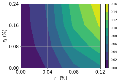
# plot contour of probability density function
x = np.linspace(low[0], high[0], 2 ** num_qubits[0])
y = np.linspace(low[1], high[1], 2 ** num_qubits[1])
z = u.probabilities.reshape(2 ** num_qubits[0], 2 ** num_qubits[1])
plt.contourf(x, y, z)
plt.xticks(x, size=15)
plt.yticks(y, size=15)
plt.grid()
plt.xlabel("$r_1$ (%)", size=15)
plt.ylabel("$r_2$ (%)", size=15)
plt.colorbar()
plt.show()
Flujo de caja, función de rendimiento, y valor esperado exacto#
A continuación, definimos el flujo de caja por periodo, la función de rendimiento resultante y evaluamos el valor esperado exacto.
Para la función de rendimiento primero utilizamos una aproximación de primer orden y luego aplicamos la misma técnica de aproximación que para la parte lineal de la función de rendimiento de la Fijación de Precios de Opciones de Compra Europeas.
[4]:
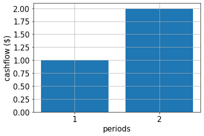
# specify cash flow
cf = [1.0, 2.0]
periods = range(1, len(cf) + 1)

# plot cash flow
plt.bar(periods, cf)
plt.xticks(periods, size=15)
plt.yticks(size=15)
plt.grid()
plt.xlabel("periods", size=15)
plt.ylabel("cashflow ($)", size=15)
plt.show()
[5]:
# estimate real value
cnt = 0
exact_value = 0.0
for x1 in np.linspace(low[0], high[0], pow(2, num_qubits[0])):
    for x2 in np.linspace(low[1], high[1], pow(2, num_qubits[1])):
        prob = u.probabilities[cnt]
        for t in range(len(cf)):
            # evaluate linear approximation of real value w.r.t. interest rates
            exact_value += prob * (
                cf[t] / pow(1 + b[t], t + 1)
                - (t + 1) * cf[t] * np.dot(A[:, t], np.asarray([x1, x2])) / pow(1 + b[t], t + 2)
            )
        cnt += 1
print("Exact value:    \t%.4f" % exact_value)
Exact value: 2.1942
[6]:
# specify approximation factor
c_approx = 0.125

# create fixed income pricing application
from qiskit_finance.applications.estimation import FixedIncomePricing

fixed_income = FixedIncomePricing(
    num_qubits=num_qubits,
    pca_matrix=A,
    initial_interests=b,
    cash_flow=cf,
    rescaling_factor=c_approx,
    bounds=bounds,
    uncertainty_model=u,
)
[7]:
fixed_income._objective.draw()
[7]:
     ┌────┐
q_0: ┤0   ├
     │    │
q_1: ┤1   ├
     │    │
q_2: ┤2 F ├
     │    │
q_3: ┤3   ├
     │    │
q_4: ┤4   ├
     └────┘
[8]:
fixed_income_circ = QuantumCircuit(fixed_income._objective.num_qubits)

# load probability distribution
fixed_income_circ.append(u, range(u.num_qubits))

# apply function
fixed_income_circ.append(fixed_income._objective, range(fixed_income._objective.num_qubits))

fixed_income_circ.draw()
[8]:
     ┌───────┐┌────┐
q_0: ┤0      ├┤0   ├
     │       ││    │
q_1: ┤1      ├┤1   ├
     │  P(X) ││    │
q_2: ┤2      ├┤2 F ├
     │       ││    │
q_3: ┤3      ├┤3   ├
     └───────┘│    │
q_4: ─────────┤4   ├
              └────┘
[9]:
# set target precision and confidence level
epsilon = 0.01
alpha = 0.05

# construct amplitude estimation
problem = fixed_income.to_estimation_problem()

ae = IterativeAmplitudeEstimation(
    epsilon_target=epsilon, alpha=alpha, sampler=Sampler(run_options={"shots": 100, "seed": 75})
)
[10]:
result = ae.estimate(problem)
[11]:
conf_int = np.array(result.confidence_interval_processed)
print("Exact value:        \t%.4f" % exact_value)
print("Estimated value:    \t%.4f" % (fixed_income.interpret(result)))
print("Confidence interval:\t[%.4f, %.4f]" % tuple(conf_int))
Exact value:            2.1942
Estimated value:        2.3437
Confidence interval:    [2.3101, 2.3772]
[12]:
import qiskit.tools.jupyter

%qiskit_version_table
%qiskit_copyright
Version Information
| Software | Version |
|---|---|
qiskit | None |
qiskit-terra | 0.45.0.dev0+c626be7 |
qiskit_finance | 0.4.0 |
qiskit_algorithms | 0.2.0 |
qiskit_ibm_provider | 0.6.1 |
qiskit_optimization | 0.6.0 |
qiskit_aer | 0.12.0 |
| System information | |
| Python version | 3.9.7 |
| Python compiler | GCC 7.5.0 |
| Python build | default, Sep 16 2021 13:09:58 |
| OS | Linux |
| CPUs | 2 |
| Memory (Gb) | 5.778430938720703 |
| Fri Aug 18 16:21:18 2023 EDT | |
This code is a part of Qiskit
© Copyright IBM 2017, 2023.
This code is licensed under the Apache License, Version 2.0. You may
obtain a copy of this license in the LICENSE.txt file in the root directory
of this source tree or at http://www.apache.org/licenses/LICENSE-2.0.
Any modifications or derivative works of this code must retain this
copyright notice, and modified files need to carry a notice indicating
that they have been altered from the originals.
[ ]: