Nota
Esta página fue generada a partir de docs/tutorials/07_asian_barrier_spread_pricing.ipynb.
Fijación de Precios de Márgenes de Barrera Asiáticos#
Introducción#
Un margen de barrera asiático es una combinación de 3 tipos de opciones diferentes y, como tal, combina múltiples características posibles que soporta el framework de precios de opciones de Qiskit Finance:
Opción asiática: La recompensa depende del precio medio durante el horizonte temporal considerado.
Opción de Barrera: La recompensa es cero si se excede un cierto umbral en cualquier momento dentro del horizonte de tiempo considerado.
Margen (Alcista): La recompensa sigue una función lineal por partes (dependiendo del precio promedio) que comienza en cero, aumenta de forma lineal y se mantiene constante.
Supón precios de ejercicio \(K_1 < K_2\) y períodos de tiempo \(t=1,2\), con los precios al contado correspondientes \((S_1, S_2)\) siguiendo una distribución multivariante dada (por ejemplo, generada por algún proceso estocástico), y un umbral de barrera \(B>0\). La función de rendimiento correspondiente se define como
A continuación, se utiliza un algoritmo cuántico basado en la estimación de amplitud para estimar el rendimiento esperado, es decir, el precio justo antes del descuento, para la opción
La aproximación de la función objetivo y una introducción general a la fijación de precios de opciones y el análisis de riesgos en computadoras cuánticas se dan en los siguientes artículos:
[1]:
import matplotlib.pyplot as plt
from scipy.interpolate import griddata

%matplotlib inline
import numpy as np

from qiskit import QuantumRegister, QuantumCircuit, AncillaRegister, transpile
from qiskit.circuit.library import IntegerComparator, WeightedAdder, LinearAmplitudeFunction
from qiskit_algorithms import IterativeAmplitudeEstimation, EstimationProblem
from qiskit_aer.primitives import Sampler
from qiskit_finance.circuit.library import LogNormalDistribution
Modelo de Incertidumbre#
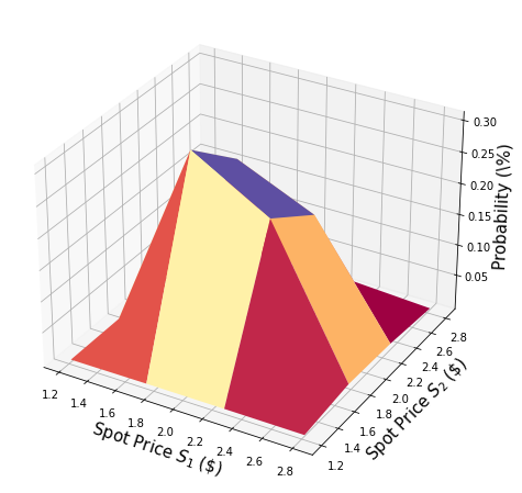
Construimos un circuito para cargar una distribución aleatoria logarítmica normal multivariante en un estado cuántico en \(n\) qubits. Para cada dimensión \(j = 1,\ldots,d\), la distribución es truncada a un intervalo dado \([\text{low}_j, \text{high}_j]\) y discretizada usando una cuadrícula de \(2^{n_j}\) puntos, donde \(n_j\) denota el número de qubits usados para representar la dimensión \(j\), es decir, \(n_1+\ldots+n_d = n\). El operador unitario correspondiente al circuito implementa lo siguiente:
donde \(p_{i_1\ldots i_d}\) denota las probabilidades correspondientes a la distribución truncada y discretizada y donde \(i_j\) se asigna al intervalo correcto usando el mapa afín:
Por simplicidad, suponemos que ambos precios de las acciones son independientes y están distribuidos de manera idéntica. Esta suposición simplemente simplifica la parametrización a continuación y se puede relajar fácilmente a distribuciones multivariadas más complejas y también correlacionadas. La única suposición importante para la implementación actual es que la cuadrícula de discretización de las diferentes dimensiones tiene el mismo tamaño de paso.
[2]:
# number of qubits per dimension to represent the uncertainty
num_uncertainty_qubits = 2

# parameters for considered random distribution
S = 2.0  # initial spot price
vol = 0.4  # volatility of 40%
r = 0.05  # annual interest rate of 4%
T = 40 / 365  # 40 days to maturity

# resulting parameters for log-normal distribution
mu = (r - 0.5 * vol**2) * T + np.log(S)
sigma = vol * np.sqrt(T)
mean = np.exp(mu + sigma**2 / 2)
variance = (np.exp(sigma**2) - 1) * np.exp(2 * mu + sigma**2)
stddev = np.sqrt(variance)

# lowest and highest value considered for the spot price; in between, an equidistant discretization is considered.
low = np.maximum(0, mean - 3 * stddev)
high = mean + 3 * stddev

# map to higher dimensional distribution
# for simplicity assuming dimensions are independent and identically distributed)
dimension = 2
num_qubits = [num_uncertainty_qubits] * dimension
low = low * np.ones(dimension)
high = high * np.ones(dimension)
mu = mu * np.ones(dimension)
cov = sigma**2 * np.eye(dimension)

# construct circuit
u = LogNormalDistribution(num_qubits=num_qubits, mu=mu, sigma=cov, bounds=(list(zip(low, high))))
[3]:
# plot PDF of uncertainty model
x = [v[0] for v in u.values]
y = [v[1] for v in u.values]
z = u.probabilities
# z = map(float, z)
# z = list(map(float, z))
resolution = np.array([2**n for n in num_qubits]) * 1j
grid_x, grid_y = np.mgrid[min(x) : max(x) : resolution[0], min(y) : max(y) : resolution[1]]
grid_z = griddata((x, y), z, (grid_x, grid_y))
plt.figure(figsize=(10, 8))
ax = plt.axes(projection="3d")
ax.plot_surface(grid_x, grid_y, grid_z, cmap=plt.cm.Spectral)
ax.set_xlabel("Spot Price $S_1$ (\$)", size=15)
ax.set_ylabel("Spot Price $S_2$ (\$)", size=15)
ax.set_zlabel("Probability (\%)", size=15)
plt.show()
Función de Rendimiento#
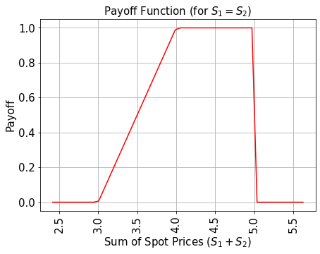
Para simplificar, consideramos la suma de los precios al contado en lugar de su promedio. El resultado se puede transformar al promedio simplemente dividiéndolo entre 2.
La función de rendimiento es igual a cero siempre que la suma de los precios al contado \((S_1 + S_2)\) sea menor que el precio de ejercicio \(K_1\) y luego aumenta linealmente hasta que la suma de los precios al contado alcanza \(K_2\). Luego, el rendimiento permanece constante en \(K_2 - K_1\) a menos que cualquiera de los dos precios al contado exceda el umbral de barrera \(B\), entonces el rendimiento baja inmediatamente a cero. La implementación primero usa un operador de suma ponderada para calcular la suma de los precios al contado en un registro ancilla, y luego usa un comparador, que cambia un qubit ancilla de \(\big|0\rangle\) a \(\big|1\rangle\) si \((S_1 + S_2) \geq K_1\) y otro comparador/ancilla para capturar el caso de que \((S_1 + S_2) \geq K_2\). Estas ancillas se utilizan para controlar la parte lineal de la función de rendimiento.
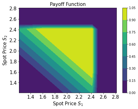
Además, agregamos otra variable auxiliar para cada paso de tiempo y usamos comparadores adicionales para verificar si \(S_1\), respectivamente \(S_2\), excede el umbral de barrera \(B\). La función de rendimiento solo se aplica si \(S_1, S_2 \leq B\).
La parte lineal en sí se aproxima de la siguiente manera. Aprovechamos el hecho de que \(\sin^2(y + \pi/4) \approx y + 1/2\) para pequeños \(|y|\). Por lo tanto, para un factor de escala de aproximación dado \(c_\text{approx} \in [0, 1]\) y \(x \in [0, 1]\) consideramos
para pequeños \(c_\text{approx}\).
Podemos construir fácilmente un operador que actúe como
utilizando rotaciones Y controladas.
Finalmente, nos interesa la probabilidad de medir \(\big|1\rangle\) en el último qubit, que corresponde a \(\sin^2(a*x+b)\). Junto con la aproximación anterior, esto permite aproximar los valores de interés. Cuanto más pequeño elijamos \(c_\text{approx}\), mejor será la aproximación. Sin embargo, dado que estamos estimando una propiedad escalada por \(c_\text{approx}\), el número de qubits de evaluación \(m\) debe ajustarse en consecuencia.
Para más detalles sobre la aproximación, nos referimos a: Quantum Risk Analysis. Woerner, Egger. 2018.
Dado que el operador de suma ponderada (en su implementación actual) solo puede sumar números enteros, necesitamos mapear desde los rangos originales al rango representable para estimar el resultado y revertir este mapeo antes de interpretar el resultado. El mapeo corresponde esencialmente al mapeo afín descrito en el contexto del modelo de incertidumbre anterior.
[4]:
# determine number of qubits required to represent total loss
weights = []
for n in num_qubits:
    for i in range(n):
        weights += [2**i]

# create aggregation circuit
agg = WeightedAdder(sum(num_qubits), weights)
n_s = agg.num_sum_qubits
n_aux = agg.num_qubits - n_s - agg.num_state_qubits  # number of additional qubits
[5]:
# set the strike price (should be within the low and the high value of the uncertainty)
strike_price_1 = 3
strike_price_2 = 4

# set the barrier threshold
barrier = 2.5

# map strike prices and barrier threshold from [low, high] to {0, ..., 2^n-1}
max_value = 2**n_s - 1
low_ = low[0]
high_ = high[0]

mapped_strike_price_1 = (
    (strike_price_1 - dimension * low_) / (high_ - low_) * (2**num_uncertainty_qubits - 1)
)
mapped_strike_price_2 = (
    (strike_price_2 - dimension * low_) / (high_ - low_) * (2**num_uncertainty_qubits - 1)
)
mapped_barrier = (barrier - low) / (high - low) * (2**num_uncertainty_qubits - 1)
[6]:
# condition and condition result
conditions = []
barrier_thresholds = [2] * dimension
n_aux_conditions = 0
for i in range(dimension):
    # target dimension of random distribution and corresponding condition (which is required to be True)
    comparator = IntegerComparator(num_qubits[i], mapped_barrier[i] + 1, geq=False)
    n_aux_conditions = max(n_aux_conditions, comparator.num_ancillas)
    conditions += [comparator]
[7]:
# set the approximation scaling for the payoff function
c_approx = 0.25

# setup piecewise linear objective fcuntion
breakpoints = [0, mapped_strike_price_1, mapped_strike_price_2]
slopes = [0, 1, 0]
offsets = [0, 0, mapped_strike_price_2 - mapped_strike_price_1]
f_min = 0
f_max = mapped_strike_price_2 - mapped_strike_price_1
objective = LinearAmplitudeFunction(
    n_s,
    slopes,
    offsets,
    domain=(0, max_value),
    image=(f_min, f_max),
    rescaling_factor=c_approx,
    breakpoints=breakpoints,
)
[8]:
# define overall multivariate problem
qr_state = QuantumRegister(u.num_qubits, "state")  # to load the probability distribution
qr_obj = QuantumRegister(1, "obj")  # to encode the function values
ar_sum = AncillaRegister(n_s, "sum")  # number of qubits used to encode the sum
ar_cond = AncillaRegister(len(conditions) + 1, "conditions")
ar = AncillaRegister(
    max(n_aux, n_aux_conditions, objective.num_ancillas), "work"
)  # additional qubits

objective_index = u.num_qubits

# define the circuit
asian_barrier_spread = QuantumCircuit(qr_state, qr_obj, ar_cond, ar_sum, ar)

# load the probability distribution
asian_barrier_spread.append(u, qr_state)

# apply the conditions
for i, cond in enumerate(conditions):
    state_qubits = qr_state[(num_uncertainty_qubits * i) : (num_uncertainty_qubits * (i + 1))]
    asian_barrier_spread.append(cond, state_qubits + [ar_cond[i]] + ar[: cond.num_ancillas])

# aggregate the conditions on a single qubit
asian_barrier_spread.mcx(ar_cond[:-1], ar_cond[-1])

# apply the aggregation function controlled on the condition
asian_barrier_spread.append(agg.control(), [ar_cond[-1]] + qr_state[:] + ar_sum[:] + ar[:n_aux])

# apply the payoff function
asian_barrier_spread.append(objective, ar_sum[:] + qr_obj[:] + ar[: objective.num_ancillas])

# uncompute the aggregation
asian_barrier_spread.append(
    agg.inverse().control(), [ar_cond[-1]] + qr_state[:] + ar_sum[:] + ar[:n_aux]
)

# uncompute the conditions
asian_barrier_spread.mcx(ar_cond[:-1], ar_cond[-1])

for j, cond in enumerate(reversed(conditions)):
    i = len(conditions) - j - 1
    state_qubits = qr_state[(num_uncertainty_qubits * i) : (num_uncertainty_qubits * (i + 1))]
    asian_barrier_spread.append(
        cond.inverse(), state_qubits + [ar_cond[i]] + ar[: cond.num_ancillas]
    )

print(asian_barrier_spread.draw())
print("objective qubit index", objective_index)
              ┌───────┐┌──────┐             ┌───────────┐      ┌──────────────┐»
     state_0: ┤0      ├┤0     ├─────────────┤1          ├──────┤1             ├»
              │       ││      │             │           │      │              │»
     state_1: ┤1      ├┤1     ├─────────────┤2          ├──────┤2             ├»
              │  P(X) ││      │┌──────┐     │           │      │              │»
     state_2: ┤2      ├┤      ├┤0     ├─────┤3          ├──────┤3             ├»
              │       ││      ││      │     │           │      │              │»
     state_3: ┤3      ├┤      ├┤1     ├─────┤4          ├──────┤4             ├»
              └───────┘│      ││      │     │           │┌────┐│              │»
         obj: ─────────┤      ├┤      ├─────┤           ├┤3   ├┤              ├»
                       │      ││      │     │           ││    ││              │»
conditions_0: ─────────┤2     ├┤      ├──■──┤           ├┤    ├┤              ├»
                       │  cmp ││      │  │  │           ││    ││              │»
conditions_1: ─────────┤      ├┤2     ├──■──┤           ├┤    ├┤              ├»
                       │      ││  cmp │┌─┴─┐│   c_adder ││    ││   c_adder_dg │»
conditions_2: ─────────┤      ├┤      ├┤ X ├┤0          ├┤    ├┤0             ├»
                       │      ││      │└───┘│           ││    ││              │»
       sum_0: ─────────┤      ├┤      ├─────┤5          ├┤0   ├┤5             ├»
                       │      ││      │     │           ││  F ││              │»
       sum_1: ─────────┤      ├┤      ├─────┤6          ├┤1   ├┤6             ├»
                       │      ││      │     │           ││    ││              │»
       sum_2: ─────────┤      ├┤      ├─────┤7          ├┤2   ├┤7             ├»
                       │      ││      │     │           ││    ││              │»
      work_0: ─────────┤3     ├┤3     ├─────┤8          ├┤4   ├┤8             ├»
                       └──────┘└──────┘     │           ││    ││              │»
      work_1: ──────────────────────────────┤9          ├┤5   ├┤9             ├»
                                            │           ││    ││              │»
      work_2: ──────────────────────────────┤10         ├┤6   ├┤10            ├»
                                            └───────────┘└────┘└──────────────┘»
«                              ┌─────────┐
«     state_0: ────────────────┤0        ├
«                              │         │
«     state_1: ────────────────┤1        ├
«                   ┌─────────┐│         │
«     state_2: ─────┤0        ├┤         ├
«                   │         ││         │
«     state_3: ─────┤1        ├┤         ├
«                   │         ││         │
«         obj: ─────┤         ├┤         ├
«                   │         ││         │
«conditions_0: ──■──┤         ├┤2        ├
«                │  │         ││  cmp_dg │
«conditions_1: ──■──┤2        ├┤         ├
«              ┌─┴─┐│  cmp_dg ││         │
«conditions_2: ┤ X ├┤         ├┤         ├
«              └───┘│         ││         │
«       sum_0: ─────┤         ├┤         ├
«                   │         ││         │
«       sum_1: ─────┤         ├┤         ├
«                   │         ││         │
«       sum_2: ─────┤         ├┤         ├
«                   │         ││         │
«      work_0: ─────┤3        ├┤3        ├
«                   └─────────┘└─────────┘
«      work_1: ───────────────────────────
«
«      work_2: ───────────────────────────
«
objective qubit index 4
[9]:
# plot exact payoff function
plt.figure(figsize=(7, 5))
x = np.linspace(sum(low), sum(high))
y = (x <= 5) * np.minimum(np.maximum(0, x - strike_price_1), strike_price_2 - strike_price_1)
plt.plot(x, y, "r-")
plt.grid()
plt.title("Payoff Function (for $S_1 = S_2$)", size=15)
plt.xlabel("Sum of Spot Prices ($S_1 + S_2)$", size=15)
plt.ylabel("Payoff", size=15)
plt.xticks(size=15, rotation=90)
plt.yticks(size=15)
plt.show()
[10]:
# plot contour of payoff function with respect to both time steps, including barrier
plt.figure(figsize=(7, 5))
z = np.zeros((17, 17))
x = np.linspace(low[0], high[0], 17)
y = np.linspace(low[1], high[1], 17)
for i, x_ in enumerate(x):
    for j, y_ in enumerate(y):
        z[i, j] = np.minimum(
            np.maximum(0, x_ + y_ - strike_price_1), strike_price_2 - strike_price_1
        )
        if x_ > barrier or y_ > barrier:
            z[i, j] = 0

plt.title("Payoff Function", size=15)
plt.contourf(x, y, z)
plt.colorbar()
plt.xlabel("Spot Price $S_1$", size=15)
plt.ylabel("Spot Price $S_2$", size=15)
plt.xticks(size=15)
plt.yticks(size=15)
plt.show()
[11]:
# evaluate exact expected value
sum_values = np.sum(u.values, axis=1)
payoff = np.minimum(np.maximum(sum_values - strike_price_1, 0), strike_price_2 - strike_price_1)
leq_barrier = [np.max(v) <= barrier for v in u.values]
exact_value = np.dot(u.probabilities[leq_barrier], payoff[leq_barrier])
print("exact expected value:\t%.4f" % exact_value)
exact expected value: 0.8023
Evaluar el Rendimiento Esperado#
Primero verificamos el circuito cuántico simulándolo y analizando la probabilidad resultante para medir el estado \(|1\rangle\) en el qubit objetivo.
[12]:
num_state_qubits = asian_barrier_spread.num_qubits - asian_barrier_spread.num_ancillas
print("state qubits: ", num_state_qubits)
transpiled = transpile(asian_barrier_spread, basis_gates=["u", "cx"])
print("circuit width:", transpiled.width())
print("circuit depth:", transpiled.depth())
state qubits:  5
circuit width: 14
circuit depth: 6373
[13]:
asian_barrier_spread_measure = asian_barrier_spread.measure_all(inplace=False)
sampler = Sampler()
job = sampler.run(asian_barrier_spread_measure)
[14]:
# evaluate the result
value = 0
probabilities = job.result().quasi_dists[0].binary_probabilities()
for i, prob in probabilities.items():
    if prob > 1e-4 and i[-num_state_qubits:][0] == "1":
        value += prob


# map value to original range
mapped_value = objective.post_processing(value) / (2**num_uncertainty_qubits - 1) * (high_ - low_)
print("Exact Operator Value:  %.4f" % value)
print("Mapped Operator value: %.4f" % mapped_value)
print("Exact Expected Payoff: %.4f" % exact_value)
Exact Operator Value:  0.6455
Mapped Operator value: 0.8705
Exact Expected Payoff: 0.8023
A continuación, usamos la estimación de amplitud para estimar el rendimiento esperado. Ten en cuenta que esto puede llevar un tiempo ya que estamos simulando una gran cantidad de qubits. La forma en que diseñamos el operador (asian_barrier_spread) implica que el número de qubits de estado reales es significativamente menor, lo que ayuda a reducir un poco el tiempo de simulación general.
[15]:
# set target precision and confidence level
epsilon = 0.01
alpha = 0.05

problem = EstimationProblem(
    state_preparation=asian_barrier_spread,
    objective_qubits=[objective_index],
    post_processing=objective.post_processing,
)
# construct amplitude estimation
ae = IterativeAmplitudeEstimation(
    epsilon, alpha=alpha, sampler=Sampler(run_options={"shots": 100, "seed": 75})
)
[16]:
result = ae.estimate(problem)
[17]:
conf_int = (
    np.array(result.confidence_interval_processed)
    / (2**num_uncertainty_qubits - 1)
    * (high_ - low_)
)
print("Exact value:    \t%.4f" % exact_value)
print(
    "Estimated value:\t%.4f"
    % (result.estimation_processed / (2**num_uncertainty_qubits - 1) * (high_ - low_))
)
print("Confidence interval: \t[%.4f, %.4f]" % tuple(conf_int))
Exact value:            0.8023
Estimated value:        0.8320
Confidence interval:    [0.8264, 0.8376]
[18]:
import qiskit.tools.jupyter

%qiskit_version_table
%qiskit_copyright
Version Information
| Software | Version |
|---|---|
qiskit | None |
qiskit-terra | 0.45.0.dev0+c626be7 |
qiskit_aer | 0.12.0 |
qiskit_ibm_provider | 0.6.1 |
qiskit_algorithms | 0.2.0 |
qiskit_finance | 0.4.0 |
| System information | |
| Python version | 3.9.7 |
| Python compiler | GCC 7.5.0 |
| Python build | default, Sep 16 2021 13:09:58 |
| OS | Linux |
| CPUs | 2 |
| Memory (Gb) | 5.778430938720703 |
| Fri Aug 18 16:20:04 2023 EDT | |
This code is a part of Qiskit
© Copyright IBM 2017, 2023.
This code is licensed under the Apache License, Version 2.0. You may
obtain a copy of this license in the LICENSE.txt file in the root directory
of this source tree or at http://www.apache.org/licenses/LICENSE-2.0.
Any modifications or derivative works of this code must retain this
copyright notice, and modified files need to carry a notice indicating
that they have been altered from the originals.
[ ]: