Quantum State Tomography#
Quantum tomography is an experimental procedure to reconstruct a description of part of a quantum system from the measurement outcomes of a specific set of experiments. In particular, quantum state tomography reconstructs the density matrix of a quantum state by preparing the state many times and measuring them in a tomographically complete basis of measurement operators.
Note
This tutorial requires the qiskit-aer and qiskit-ibm-runtime
packages to run simulations. You can install them with python -m pip
install qiskit-aer qiskit-ibm-runtime.
We first initialize a simulator to run the experiments on.
from qiskit_aer import AerSimulator
from qiskit_ibm_runtime.fake_provider import FakePerth

backend = AerSimulator.from_backend(FakePerth())
To run a state tomography experiment, we initialize the experiment with a circuit to
prepare the state to be measured. We can also pass in an
Operator or a Statevector
to describe the preparation circuit.
import qiskit
from qiskit_experiments.framework import ParallelExperiment
from qiskit_experiments.library import StateTomography

# GHZ State preparation circuit
nq = 2
qc_ghz = qiskit.QuantumCircuit(nq)
qc_ghz.h(0)
qc_ghz.s(0)
for i in range(1, nq):
    qc_ghz.cx(0, i)

# QST Experiment
qstexp1 = StateTomography(qc_ghz)
qstdata1 = qstexp1.run(backend, seed_simulation=100).block_for_results()

# Print results
for result in qstdata1.analysis_results():
    print(result)
AnalysisResult
- name: state
- value: DensityMatrix([[ 4.66308594e-01+0.j        ,  1.36718750e-02-0.01757812j,
                 3.25520833e-04-0.00130208j,  2.44140625e-03-0.453125j  ],
               [ 1.36718750e-02+0.01757812j,  2.39257813e-02+0.j        ,
                 1.51367188e-02-0.00390625j,  5.20833333e-03-0.00911458j],
               [ 3.25520833e-04+0.00130208j,  1.51367188e-02+0.00390625j,
                 2.29492188e-02+0.j        , -1.36718750e-02+0.00585937j],
               [ 2.44140625e-03+0.453125j  ,  5.20833333e-03+0.00911458j,
                -1.36718750e-02-0.00585937j,  4.86816406e-01+0.j        ]],
              dims=(2, 2))
- quality: unknown
- extra: <9 items>
- device_components: ['Q0', 'Q1']
- verified: False
AnalysisResult
- name: state_fidelity
- value: 0.9296874999999996
- quality: unknown
- extra: <9 items>
- device_components: ['Q0', 'Q1']
- verified: False
AnalysisResult
- name: positive
- value: True
- quality: unknown
- extra: <9 items>
- device_components: ['Q0', 'Q1']
- verified: False
Tomography Results#
The main result for tomography is the fitted state, which is stored as a
DensityMatrix object:
state_result = qstdata1.analysis_results("state")
print(state_result.value)
DensityMatrix([[ 4.66308594e-01+0.j        ,  1.36718750e-02-0.01757812j,
                 3.25520833e-04-0.00130208j,  2.44140625e-03-0.453125j  ],
               [ 1.36718750e-02+0.01757812j,  2.39257813e-02+0.j        ,
                 1.51367188e-02-0.00390625j,  5.20833333e-03-0.00911458j],
               [ 3.25520833e-04+0.00130208j,  1.51367188e-02+0.00390625j,
                 2.29492188e-02+0.j        , -1.36718750e-02+0.00585937j],
               [ 2.44140625e-03+0.453125j  ,  5.20833333e-03+0.00911458j,
                -1.36718750e-02-0.00585937j,  4.86816406e-01+0.j        ]],
              dims=(2, 2))
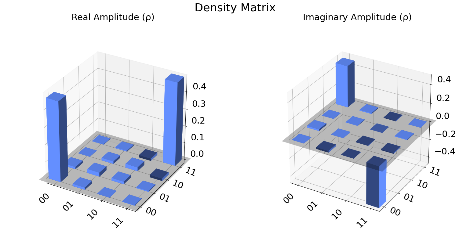
We can also visualize the density matrix:
from qiskit.visualization import plot_state_city
plot_state_city(qstdata1.analysis_results("state").value, title='Density Matrix')
The state fidelity of the fitted state with the ideal state prepared by
the input circuit is stored in the "state_fidelity" result field.
Note that if the input circuit contained any measurements the ideal
state cannot be automatically generated and this field will be set to
None.
fid_result = qstdata1.analysis_results("state_fidelity")
print("State Fidelity = {:.5f}".format(fid_result.value))
State Fidelity = 0.92969
Additional state metadata#
Additional data is stored in the tomography under the
"state_metadata" field. This includes
eigvals: the eigenvalues of the fitted statetrace: the trace of the fitted statepositive: Whether the eigenvalues are all non-negativepositive_delta: the deviation from positivity given by 1-norm of negative eigenvalues.
If trace rescaling was performed this dictionary will also contain a raw_trace field
containing the trace before rescaling. Futhermore, if the state was rescaled to be
positive or trace 1 an additional field raw_eigvals will contain the state
eigenvalues before rescaling was performed.
state_result.extra
{'trace': 1.0000000000000018,
 'eigvals': array([0.93047325, 0.04778345, 0.01514085, 0.00660245]),
 'raw_eigvals': array([0.93047325, 0.04778345, 0.01514085, 0.00660245]),
 'rescaled_psd': False,
 'fitter_metadata': {'fitter': 'linear_inversion',
  'fitter_time': 0.009145736694335938},
 'conditional_probability': 1.0,
 'positive': True,
 'experiment': 'StateTomography',
 'run_time': None}
To see the effect of rescaling, we can perform a “bad” fit with very low counts:
# QST Experiment
bad_data = qstexp1.run(backend, shots=10, seed_simulation=100).block_for_results()
bad_state_result = bad_data.analysis_results("state")

# Print result
print(bad_state_result)

# Show extra data
bad_state_result.extra
AnalysisResult
- name: state
- value: DensityMatrix([[ 0.4182829 +0.00000000e+00j, -0.0506988 +2.22733398e-04j,
                -0.07735414-1.68176592e-01j,  0.08275743-4.42318276e-01j],
               [-0.0506988 -2.22733398e-04j,  0.01349786-2.16840434e-19j,
                 0.00830736+1.92492721e-02j, -0.01133453+5.71181222e-02j],
               [-0.07735414+1.68176592e-01j,  0.00830736-1.92492721e-02j,
                 0.08224155+0.00000000e+00j,  0.16211018+1.14429332e-01j],
               [ 0.08275743+4.42318276e-01j, -0.01133453-5.71181222e-02j,
                 0.16211018-1.14429332e-01j,  0.48597768+0.00000000e+00j]],
              dims=(2, 2))
- quality: unknown
- extra: <9 items>
- device_components: ['Q0', 'Q1']
- verified: False
{'trace': 1.0000000000000013,
 'eigvals': array([0.99150418, 0.00849582, 0.        , 0.        ]),
 'raw_eigvals': array([ 1.06229031,  0.07928196, -0.0253923 , -0.11617997]),
 'rescaled_psd': True,
 'fitter_metadata': {'fitter': 'linear_inversion',
  'fitter_time': 0.004891633987426758},
 'conditional_probability': 1.0,
 'positive': True,
 'experiment': 'StateTomography',
 'run_time': None}
Tomography Fitters#
The default fitters is linear_inversion, which reconstructs the
state using dual basis of the tomography basis. This will typically
result in a non-positive reconstructed state. This state is rescaled to
be positive-semidefinite (PSD) by computing its eigen-decomposition and
rescaling its eigenvalues using the approach from Ref. [1].
There are several other fitters are included (See API documentation for
details). For example, if cvxpy is installed we can use the
cvxpy_gaussian_lstsq() fitter, which allows constraining the fit to be
PSD without requiring rescaling.
try:
    import cvxpy

    # Set analysis option for cvxpy fitter
    qstexp1.analysis.set_options(fitter='cvxpy_gaussian_lstsq')

    # Re-run experiment
    qstdata2 = qstexp1.run(backend, seed_simulation=100).block_for_results()

    state_result2 = qstdata2.analysis_results("state")
    print(state_result2)
    print("\nextra:")
    for key, val in state_result2.extra.items():
        print(f"- {key}: {val}")

except ModuleNotFoundError:
    print("CVXPY is not installed")
AnalysisResult
- name: state
- value: DensityMatrix([[ 0.46990035+0.00000000e+00j, -0.01197756-1.72210109e-04j,
                 0.00179403+2.05609672e-03j,  0.0048193 -4.54968820e-01j],
               [-0.01197756+1.72210109e-04j,  0.03022629+0.00000000e+00j,
                 0.00779256-3.68380116e-03j, -0.0111848 -1.17118385e-02j],
               [ 0.00179403-2.05609672e-03j,  0.00779256+3.68380116e-03j,
                 0.02054639+0.00000000e+00j,  0.00614826+4.58659498e-04j],
               [ 0.0048193 +4.54968820e-01j, -0.0111848 +1.17118385e-02j,
                 0.00614826-4.58659498e-04j,  0.47932697+0.00000000e+00j]],
              dims=(2, 2))
- quality: unknown
- extra: <9 items>
- device_components: ['Q0', 'Q1']
- verified: False

extra:
- trace: 1.0000000025043012
- eigvals: [0.92971227 0.046099   0.02220922 0.00197951]
- raw_eigvals: [0.92971227 0.046099   0.02220922 0.00197951]
- rescaled_psd: False
- fitter_metadata: {'fitter': 'cvxpy_gaussian_lstsq', 'cvxpy_solver': 'SCS', 'cvxpy_status': ['optimal'], 'psd_constraint': True, 'trace_preserving': True, 'fitter_time': 0.021280765533447266}
- conditional_probability: 1.0
- positive: True
- experiment: StateTomography
- run_time: None
Parallel Tomography Experiment#
We can also use the ParallelExperiment class to
run subsystem tomography on multiple qubits in parallel.
For example if we want to perform 1-qubit QST on several qubits at once:
from math import pi
num_qubits = 5
gates = [qiskit.circuit.library.RXGate(i * pi / (num_qubits - 1))
         for i in range(num_qubits)]

subexps = [
    StateTomography(gate, physical_qubits=(i,))
    for i, gate in enumerate(gates)
]
parexp = ParallelExperiment(subexps)
pardata = parexp.run(backend, seed_simulation=100).block_for_results()

for result in pardata.analysis_results():
    print(result)
View component experiment analysis results:
for i, expdata in enumerate(pardata.child_data()):
    state_result_i = expdata.analysis_results("state")
    fid_result_i = expdata.analysis_results("state_fidelity")

    print(f'\nPARALLEL EXP {i}')
    print("State Fidelity: {:.5f}".format(fid_result_i.value))
    print("State: {}".format(state_result_i.value))
PARALLEL EXP 0
State Fidelity: 0.97754
State: DensityMatrix([[0.97753906+0.j        , 0.03125   +0.00585938j],
               [0.03125   -0.00585938j, 0.02246094+0.j        ]],
              dims=(2,))

PARALLEL EXP 1
State Fidelity: 0.98475
State: DensityMatrix([[0.84863281+0.j        , 0.02246094+0.33691406j],
               [0.02246094-0.33691406j, 0.15136719+0.j        ]],
              dims=(2,))

PARALLEL EXP 2
State Fidelity: 0.98340
State: DensityMatrix([[0.49316406+0.j        , 0.01171875+0.48339844j],
               [0.01171875-0.48339844j, 0.50683594+0.j        ]],
              dims=(2,))

PARALLEL EXP 3
State Fidelity: 0.97854
State: DensityMatrix([[ 0.16015625+0.j        , -0.00488281+0.33691406j],
               [-0.00488281-0.33691406j,  0.83984375+0.j        ]],
              dims=(2,))

PARALLEL EXP 4
State Fidelity: 0.97266
State: DensityMatrix([[0.02734375+0.j        , 0.00390625-0.00195312j],
               [0.00390625+0.00195312j, 0.97265625+0.j        ]],
              dims=(2,))
References#
See also#
API documentation:
StateTomography