AC Stark Effect

When a qubit is driven with an off-resonant tone, the qubit frequency \(f_0\) is slightly shifted through what is known as the (AC) Stark effect. This technique is sometimes used to characterize qubit properties in the vicinity of the base frequency, especially with a fixed frequency qubit architecture which otherwise doesn’t have a knob to control frequency [1].

The important control parameters of the Stark effect are the amplitude \(\Omega\) and frequency \(f_S\) of the off-resonant tone, which we will call the Stark tone in the following. In the low power limit, the amount of frequency shift \(\delta f_S\) that the qubit may experience is described as follows [2]:

\[\delta f_S \approx \frac{\alpha}{2\Delta\left(\alpha - \Delta\right)} \Omega^2,\]

where \(\alpha\) is the qubit anharmonicity and \(\Delta=f_S - f_0\) is the frequency separation of the Stark tone from the qubit frequency \(f_0\). We sometimes call \(\delta f_S\) the Stark shift [3].

Stark tone implementation in Qiskit

Usually, we fix the Stark tone frequency \(f_S\) and control the amplitude \(\Omega\) to modulate the qubit frequency. In Qiskit, we often use an abstracted amplitude \(\bar{\Omega}\), instead of the physical amplitude \(\Omega\) in the experiments.

Because the Stark shift \(\delta f_S\) has a quadratic dependence on the tone amplitude \(\Omega\), the resulting shift is not sensitive to its sign. On the other hand, the sign of the shift depends on the sign of the frequency offset \(\Delta\). In a typical parameter regime of \(|\Delta | < | \alpha |\),

\[\text{sign}(\delta f_S) = - \text{sign}(\Delta).\]

In other words, positive (negative) Stark shift occurs when the tone frequency \(f_S\) is lower (higher) than the qubit frequency \(f_0\). When an experimentalist wants to perform spectroscopy of some qubit parameter in the vicinity of \(f_0\), one must manage the sign of \(f_S\) in addition to the magnitude of \(\Omega\).

To alleviate such experimental complexity, an abstracted amplitude \(\bar{\Omega}\) with virtual sign is introduced in Qiskit Experiments. This works as follows:

\[\begin{split}\Delta &= - \text{sign}(\bar{\Omega}) | \Delta |, \\ \Omega &= | \bar{\Omega} |.\end{split}\]

Stark experiments in Qiskit usually take two control parameters \((\bar{\Omega}, |\Delta|)\), which are specified by stark_amp and stark_freq_offset in the experiment options, respectively. In this representation, the sign of the Stark shift matches the sign of \(\bar{\Omega}\).

\[\text{sign}(\delta f_S) = \text{sign}(\bar{\Omega})\]

This allows an experimentalist to control both the sign and the amount of the Stark shift with the stark_amp experiment option. Note that stark_freq_offset should be set as a positive number.

Stark tone frequency

As you can see in the equation for \(\delta f_S\) above, \(\Delta=0\) yields a singular point where \(\delta f_S\) diverges. This corresponds to a Rabi drive, where the qubit is driven on resonance and coherent state exchange occurs between \(|0\rangle\) and \(|1\rangle\) instead of the Stark shift. Another frequency that should be avoided for the Stark tone is \(\Delta=\alpha\) which corresponds to the transition from \(|1\rangle\) to \(|2\rangle\). In the high power limit, \(\Delta = \alpha/2\) should also be avoided since this causes the direct excitation from \(|0\rangle\) to \(|2\rangle\) through what is known as a two-photon transition.

The Stark tone frequency must be sufficiently separated from all of these frequencies to avoid unwanted state transitions (frequency collisions). In reality, the choice of the frequency could be even more complicated due to the transition levels of the nearest neighbor qubits. The frequency must be carefully chosen to avoid frequency collisions [4].

Stark tone channel

It may be necessary to supply a pulse channel to apply the Stark tone. In Qiskit Experiments, the Stark experiments usually have an experiment option stark_channel to specify this. By default, the Stark tone is applied to the same channel as the qubit drive with a frequency shift. This frequency shift might update the channel frame, which accumulates unwanted phase against the frequency difference between the qubit drive \(f_0\) and Stark tone frequencies \(f_S\) in addition to the qubit Stark shift \(\delta f_s\). You can use a dedicated Stark drive channel if available. Otherwise, you may want to use a control channel associated with the physical drive port of the qubit.

In a typical IBM device using the cross-resonance drive architecture, such channel can be identified with your backend as follows:

Note

This tutorial requires the qiskit-ibm-runtime package to model a backend. You can install it with python -m pip install qiskit-ibm-runtime.

from qiskit_ibm_runtime.fake_provider import FakeHanoiV2

backend = FakeHanoiV2()
qubit = 0

for qpair in backend.coupling_map:
    if qpair[0] == qubit:
        break

print(backend.control_channel(qpair)[0])

ControlChannel(0)

This returns a control channel for which the qubit is the control qubit. This approach may not work for other device architectures.

Characterizing the frequency shift

One can experimentally measure \(\delta f_S\) with the StarkRamseyXY experiment. The following pulse sequence illustrates how \(\delta f_S\) is characterized by a variant of the Hahn-echo pulse sequence [5].

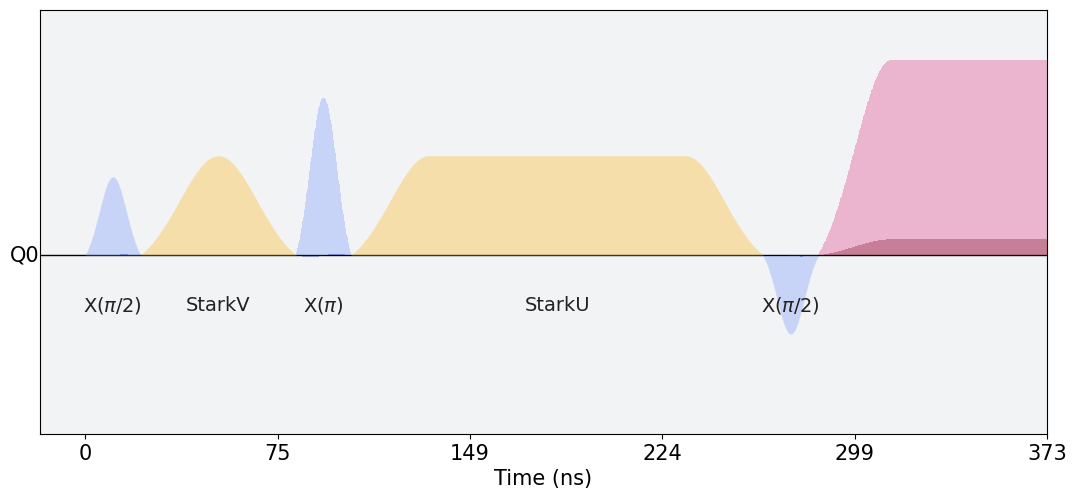
The qubit is initialized in the \(Y\)-eigenstate with the first half-pi pulse. This state may be visualized by a Bloch vector located on the equator of the Bloch sphere, which is highly sensitive to Z rotation arising from any qubit frequency offset. This operation is followed by a pi-pulse and another negative half-pi pulse right before the measurement tone filled in red. This sequence recovers the initial state when Z rotation is zero or \(\delta f_S=0\).

As you may notice, this sequence is interleaved with two pulses labeled “StarkV” (Gaussian) and “StarkU” (GaussianSquare) filled in yellow, representing Stark tones. These pulses are designed to have the same maximum amplitude \(\Omega\) resulting in the same \(\delta f_S\) at this amplitude – but why do we need two pulses?

Since \(\delta f_S\) is amplitude dependent, the Stark pulses cause time-dependent frequency shifts during the pulse ramps. With a single Stark tone, you are only able to estimate the average \(\delta f_S\) over the history of amplitudes \(\Omega(t)\), even though you may want to characterize \(\delta f_S\) at a particular \(\Omega\). You have to remember that you cannot use a square envelope to set a uniform amplitude, because the sharp rise and fall of the pulse amplitude has a broad frequency spectrum which could produce unwanted excitations.

The pulse sequence shown above is adopted to address such issue. The Z rotation accumulated by the first pulse is proportional to \(\int \Omega_V^2(t) dt\), while that of the second pulse is \(-\int \Omega_U^2(t) dt\) because the qubit state is flipped by the pi-pulse in the middle, flipping the sense of rotation of the state even though the actual rotation direction is the same for both pulses. The only difference between \(\Omega_U(t)\) and \(\Omega_V(t)\) is the flat-top part with constant amplitude \(\Omega\) and duration \(t_w\), where \(\delta f_S\) is also constant. Thanks to this sign flip, the net Z rotation \(\theta\) accumulated through the two pulses is proportional to only the flat-top part of the StarkU pulse.

\[\theta = 2 \pi \int \delta f_S(t) dt \propto \int \Omega_U^2(t) dt - \int \Omega_V^2(t) dt = \Omega^2 t_w\]

This technique allows you to estimate \(\delta f_S\) at a particular \(\Omega\).

In Qiskit Experiments, the experiment option stark_amp usually refers to the height of this GaussianSquare flat-top.

Workflow

In this example, you’ll learn how to measure a spectrum of qubit relaxation versus frequency with fixed frequency transmons. As you already know, we give an offset to the qubit frequency with a Stark tone, and the workflow starts from characterizing the amount of the Stark shift against the Stark amplitude \(\bar{\Omega}\) that you can experimentally control.

from qiskit_experiments.library.driven_freq_tuning import StarkRamseyXYAmpScan

exp = StarkRamseyXYAmpScan((0,), backend=backend)
exp_data = exp.run().block_for_results()
coefficients = exp_data.analysis_results("stark_coefficients").value

You first need to run the StarkRamseyXYAmpScan experiment that scans \(\bar{\Omega}\) and estimates the amount of the resultant frequency shift. This experiment fits the frequency shift to a polynomial model which is a function of \(\bar{\Omega}\). You can obtain the StarkCoefficients object that contains all polynomial coefficients to map and reverse-map the \(\bar{\Omega}\) to a corresponding frequency value.

This object may be necessary for the following spectroscopy experiment. Since Stark coefficients are stable for a relatively long time, you may want to save the coefficient values and load them later when you run the experiment. If you have an access to the Experiment service, you can just save the experiment result.

exp_data.save()

You can view the experiment online at https://quantum.ibm.com/experiments/23095777-be28-4036-9c98-89d3a915b820

Otherwise, you can dump the coefficient object into a file with JSON format.

import json
from qiskit_experiments.framework import ExperimentEncoder

with open("coefficients.json", "w") as fp:
    json.dump(ret_coeffs, fp, cls=ExperimentEncoder)

The saved object can be retrieved either from the service or file, as follows.

# When you have access to Experiment service
from qiskit_experiments.library.driven_freq_tuning import retrieve_coefficients_from_backend

coefficients = retrieve_coefficients_from_backend(backend, 0)

# Alternatively you can load from file
from qiskit_experiments.framework import ExperimentDecoder

with open("coefficients.json", "r") as fp:
    coefficients = json.load(fp, cls=ExperimentDecoder)

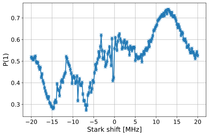
Now you can measure the qubit relaxation spectrum. The StarkP1Spectroscopy experiment also scans \(\bar{\Omega}\), but instead of measuring the frequency shift, it measures the excited state population P1 after certain delay, t1_delay in the experiment options, following the state population. You can scan the \(\bar{\Omega}\) values either in the “frequency” or “amplitude” domain, but the stark_coefficients option must be set to perform the frequency sweep.

from qiskit_experiments.library.driven_freq_tuning import StarkP1Spectroscopy

exp = StarkP1Spectroscopy((0,), backend=backend)

exp.set_experiment_options(
    t1_delay=20e-6,
    min_xval=-20e6,
    max_xval=20e6,
    xval_type="frequency",
    spacing="linear",
    stark_coefficients=coefficients,
)

exp_data = exp.run().block_for_results()

You may find notches in the P1 spectrum, which may indicate the existence of TLS’s in the vicinity of your qubit drive frequency.

exp_data.figure(0)

Note that this experiment doesn’t yield any analysis result because the landscape of a P1 spectrum can not be predicted due to the random occurrences of the TLS and frequency collisions. If you have your own protocol to extract meaningful quantities from the data, you can write a custom analysis subclass and give it to the experiment instance before execution. See StarkP1SpectAnalysis for more details.

This protocol can be parallelized among many qubits unless crosstalk matters.

References

[1]

Malcolm Carroll, Sami Rosenblatt, Petar Jurcevic, Isaac Lauer and Abhinav Kandala, Dynamics of superconducting qubit relaxation times, npj Quantum Inf 8, 132 (2022). https://arxiv.org/abs/2105.15201

[2]

Easwar Magesan, Jay M. Gambetta, Effective Hamiltonian models of the cross-resonance gate, Phys. Rev. A 101, 052308 (2020). https://arxiv.org/abs/1804.04073

[3]

Wikipedia. “Autler–Townes effect” Wikipedia Foundation. https://en.wikipedia.org/wiki/Autler%E2%80%93Townes_effect

[4]

Jared B. Hertzberg, Eric J. Zhang, Sami Rosenblatt, et. al., Laser-annealing Josephson junctions for yielding scaled-up superconducting quantum processors, npj Quantum Information 7, 129 (2021). https://arxiv.org/abs/2009.00781

[5]

J. Stehlik, D. M. Zajac, D. L. Underwood, et.al., Tunable Coupling Architecture for Fixed-Frequency Transmon Superconducting Qubits, Phys. Rev. Lett. 127, 080505 (2021). https://arxiv.org/abs/2101.07746