How-to use different array libraries and types with Qiskit Dynamics

The simulations and computations in Qiskit Dynamics can be executed with different array libraries and types. A user can choose to use either NumPy or JAX to define their models, and the code in Qiskit Dynamics will execute as if the array operations had been natively written in either library. Additionally, a user can specify that the operators in a model be stored in sparse types offered by SciPy or JAX (see configuring simulations for performance). Internally, Qiskit Dynamics utilizes Arraylias to dispatch computations on different array types to the appropriate library function.

This guide addresses the following topics:

1. Example: How-to use either NumPy or JAX when building a Signal.

2. How-to use the Qiskit Dynamics NumPy and SciPy aliased libraries.

3. How-to write JAX-transformable simulations.

1. Example: How-to use either NumPy or JAX when building a Signal

First, configure JAX and import array libraries.

# configure jax to use 64 bit mode
import jax
jax.config.update("jax_enable_x64", True)

# tell JAX we are using CPU
jax.config.update('jax_platform_name', 'cpu')

import numpy as np
import jax.numpy as jnp

Defining equivalent Signal instances, with envelope implemented in either NumPy or JAX.

from qiskit_dynamics import Signal

def envelope_numpy(t):
    return np.exp(-(t - 0.5)**2 / 0.025)

def envelope_jax(t):
    return jnp.exp(-(t - 0.5)**2 / 0.025)

signal_numpy = Signal(envelope=envelope_numpy)
signal_jax = Signal(envelope=envelope_jax)

Evaluation of signal_numpy is executed with NumPy:

type(signal_numpy(0.1))

numpy.float64

Evaluation of signal_jax is executed with JAX:

type(signal_jax(0.1))

jaxlib.xla_extension.ArrayImpl

JAX transformations can be applied to signal_jax, e.g. just-in-time compilation:

from jax import jit

jit_signal_jax = jit(signal_jax)
jit_signal_jax(0.1)

Array(0.00166156, dtype=float64)

2. How-to use the Qiskit Dynamics NumPy and SciPy aliased libraries

Internally, Qiskit Dynamics uses an extension of the default NumPy and SciPy array libraries offered by Arraylias. These can be imported as:

# alias for NumPy and corresponding aliased library
from qiskit_dynamics import DYNAMICS_NUMPY_ALIAS
from qiskit_dynamics import DYNAMICS_NUMPY

# alias for SciPy and corresponding aliased library
from qiskit_dynamics import DYNAMICS_SCIPY_ALIAS
from qiskit_dynamics import DYNAMICS_SCIPY

See the Arraylias documentation for how the general library aliasing framework works, as well as the Qiskit Dynamics submodule arraylias for a description of how the default NumPy and SciPy aliases have been extended for use in this package.

3. How-to write JAX-transformable simulations

One of the primary benefits of JAX is its function transformations; e.g. just-in-time compilation, and automatic differentiation. To make use of these transformations in Qiskit Dynamics simulations, a user needs to ensure that the user-supplied code is itself JAX-transformable (e.g. the Signal envelope defined above), and that they use a JAX-based solver.

Here, we walk through an example of building a Solver, and JAX-compiling a simulation that scans over a control parameter.

First, we construct a Solver instance with a simple qubit model.

import numpy as np
from qiskit.quantum_info import Operator
from qiskit_dynamics import Solver, Signal

r = 0.5
w = 1.
X = Operator.from_label('X')
Z = Operator.from_label('Z')

static_hamiltonian = 2 * np.pi * w * Z/2
hamiltonian_operators = [2 * np.pi * r * X/2]

solver = Solver(
    static_hamiltonian=static_hamiltonian,
    hamiltonian_operators=hamiltonian_operators,
    rotating_frame=static_hamiltonian
)

Next, define the function to be compiled:

• The input is the amplitude of a constant-envelope signal on resonance, driven over time \([0, 3]\).

• The output is the state of the system, starting in the ground state, at 100 points over the total evolution time.

def sim_function(amp):

    # define a signal with constant envelope, on resonance
    signals = [Signal(amp, carrier_freq=w)]

    # run the simulation
    results = solver.solve(
        t_span=[0, 3.],
        y0=np.array([0., 1.], dtype=complex),
        signals=signals,
        t_eval=np.linspace(0, 3., 100),
        method='jax_odeint'
    )

    return results.y

Compile the function.

from jax import jit
fast_sim = jit(sim_function)

The first time the function is called, JAX will compile an XLA version of the function, which is then executed. Hence, the time taken on the first call includes compilation time.

%time ys = fast_sim(1.).block_until_ready()

CPU times: user 561 ms, sys: 28.7 ms, total: 590 ms
Wall time: 581 ms

On subsequent calls the compiled function is directly executed, demonstrating the true speed of the compiled function.

%timeit fast_sim(1.).block_until_ready()

95.9 µs ± 203 ns per loop (mean ± std. dev. of 7 runs, 10,000 loops each)

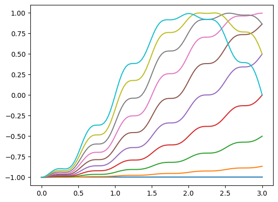
We use this function to plot the \(Z\) expectation value over a range of input amplitudes.

import matplotlib.pyplot as plt

for amp in np.linspace(0, 1, 10):
    ys = fast_sim(amp)
    plt.plot(np.linspace(0, 3., 100), np.real(np.abs(ys[:, 0])**2-np.abs(ys[:, 1])**2))