Simulating backends at the pulse-level with DynamicsBackend#
In this tutorial we walk through how to use the DynamicsBackend class as a Qiskit
Dynamics-backed, pulse-level simulator of a real backend. In particular, we demonstrate how to
configure a DynamicsBackend to simulate pulse schedules, circuits whose gates have pulse
definitions, and calibration and characterization experiments from Qiskit Experiments.
The sections of this tutorial are as follows:
Configure JAX.
Instantiating a minimally-configured
DynamicsBackendwith a 2 qubit model.Simulating pulse schedules on the
DynamicsBackend.Simulating circuits at the pulse level using the
DynamicsBackend.Simulating single-qubit calibration processes via Qiskit Experiments.
Simulating 2 qubit interaction characterization via the
CrossResonanceHamiltonianexperiment.
1. Configure JAX#
Note that the DynamicsBackend internally performs just-in-time compilation automatically
when using a JAX solver method. Here we configure JAX to run on CPU in 64 bit mode. See the
User Guide entry on using different array libraries with Qiskit Dynamics for more information.
# Configure JAX
import jax
jax.config.update("jax_enable_x64", True)
jax.config.update("jax_platform_name", "cpu")
2. Instantiating a minimally-configured DynamicsBackend with a 2 qubit model#
To create the DynamicsBackend, first specify a Solver instance using the model
details. Note that the choice of model depends on the type of device you wish to simulate. Here, we
will use a \(2\) qubit fixed-frequency transmon model with fixed coupling, with the following
Hamiltonian:
where
\(\nu_0\) and \(\nu_1\) are the qubit frequencies,
\(\alpha_0\) and \(\alpha_1\) are the qubit anharmonicities,
\(J\) is the coupling strength,
\(r_0\) and \(r_1\) are the Rabi strengths, and \(s_0(t)\) and \(s_1(t)\) are the drive signals,
\(a_j\) and \(a_j^\dagger\) are the lowering and raising operators for qubit \(j\), and
\(N_0\) and \(N_1\) are the number operators for qubits \(0\) and \(1\) respectively.
import numpy as np

dim = 3

v0 = 4.86e9
anharm0 = -0.32e9
r0 = 0.22e9

v1 = 4.97e9
anharm1 = -0.32e9
r1 = 0.26e9

J = 0.002e9

a = np.diag(np.sqrt(np.arange(1, dim)), 1)
adag = np.diag(np.sqrt(np.arange(1, dim)), -1)
N = np.diag(np.arange(dim))

ident = np.eye(dim, dtype=complex)
full_ident = np.eye(dim**2, dtype=complex)

N0 = np.kron(ident, N)
N1 = np.kron(N, ident)

a0 = np.kron(ident, a)
a1 = np.kron(a, ident)

a0dag = np.kron(ident, adag)
a1dag = np.kron(adag, ident)


static_ham0 = 2 * np.pi * v0 * N0 + np.pi * anharm0 * N0 * (N0 - full_ident)
static_ham1 = 2 * np.pi * v1 * N1 + np.pi * anharm1 * N1 * (N1 - full_ident)

static_ham_full = static_ham0 + static_ham1 + 2 * np.pi * J * ((a0 + a0dag) @ (a1 + a1dag))

drive_op0 = 2 * np.pi * r0 * (a0 + a0dag)
drive_op1 = 2 * np.pi * r1 * (a1 + a1dag)
Construct the Solver using the model details, including parameters necessary for pulse
simulation. See the Solver documentation, as well as the tutorial example for more details. Here, we choose to perform the simulation in the rotating frame of the
static Hamiltonian, which provides performance improvements (see the user guide entry on
configuring simulations for performance). Note that the measurement
outcomes of DynamicsBackend.run() are independent of the choice of rotating frame in the
Solver, and as such we are free to choose the rotating frame that provides the best
performance.
from qiskit_dynamics import Solver

# build solver
dt = 1/4.5e9

solver = Solver(
    static_hamiltonian=static_ham_full,
    hamiltonian_operators=[drive_op0, drive_op1, drive_op0, drive_op1],
    rotating_frame=static_ham_full,
    hamiltonian_channels=["d0", "d1", "u0", "u1"],
    channel_carrier_freqs={"d0": v0, "d1": v1, "u0": v1, "u1": v0},
    dt=dt,
    array_library="jax",
)
Next, instantiate the DynamicsBackend. The solver is used for simulation,
subsystem_dims indicates how the full system decomposes for measurement data computation, and
solver_options are consistent options used by Solver.solve() when simulating the
differential equation. The full list of allowable solver_options are the arguments to
solve_ode().
Note that, to enable the internal automatic jit-compilation, we choose a JAX integration method.
Furthermore, note that in the solver options we set the max step size to the pulse sample width
dt via the "hmax" argument for the method "jax_odeint". This is important for preventing
variable step solvers from accidentally stepping over pulses in schedules with long idle times.
from qiskit_dynamics import DynamicsBackend

# Consistent solver option to use throughout notebook
solver_options = {"method": "jax_odeint", "atol": 1e-6, "rtol": 1e-8, "hmax": dt}

backend = DynamicsBackend(
    solver=solver,
    subsystem_dims=[dim, dim], # for computing measurement data
    solver_options=solver_options, # to be used every time run is called
)
Alternatively to the above, the DynamicsBackend.from_backend() method can be used to build
the DynamicsBackend from an existing backend. The above model, which was built manually,
was taken from qubits \(0\) and \(1\) of almaden.
3. Simulating pulse schedules on the DynamicsBackend#
With the above backend, we can already simulate a list of pulse schedules. The code below generates
a list of schedules specifying experiments on qubit \(0\). The schedule is chosen to demonstrate
that the usual instructions work on the DynamicsBackend.
Note
In the following constructed schedule, measurement is performed with an
Acquire instruction of duration 1. Measurements in
DynamicsBackend are computed projectively at the start time of the acquire
instructions, and the effects of measurement stimulus through
MeasureChannels are not simulated unless explicitly put into
the model by the user. As such, the lack of MeasureChannel
stimulus, and the duration of the Acquire instruction has no
impact on the returned results.
%%time

from qiskit import pulse

sigma = 128
num_samples = 256

schedules = []

for amp in np.linspace(0., 1., 10):
    gauss = pulse.library.Gaussian(
        num_samples, amp, sigma, name="Parametric Gauss"
    )

    with pulse.build() as schedule:
        with pulse.align_sequential():
            pulse.play(gauss, pulse.DriveChannel(0))
            pulse.shift_phase(0.5, pulse.DriveChannel(0))
            pulse.shift_frequency(0.1, pulse.DriveChannel(0))
            pulse.play(gauss, pulse.DriveChannel(0))
            pulse.acquire(duration=1, qubit_or_channel=0, register=pulse.MemorySlot(0))

    schedules.append(schedule)

job = backend.run(schedules, shots=100)
result = job.result()
CPU times: user 1.23 s, sys: 152 ms, total: 1.38 s
Wall time: 1.41 s
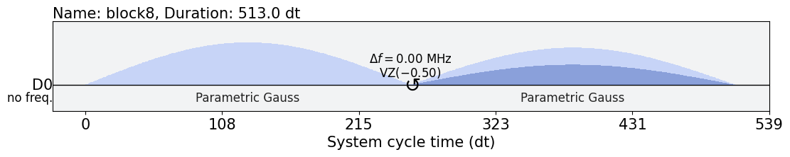
Visualize one of the schedules.
schedules[3].draw()
Retrieve the counts for one of the experiments as would be done using the results object from a real backend.
result.get_counts(3)
{'0': 50, '1': 50}
4. Simulating circuits at the pulse level using the DynamicsBackend#
For the DynamicsBackend to simulate a circuit, each circuit element must have a
corresponding pulse schedule. These schedules can either be specified in the gates themselves, by
attaching calibrations, or by adding instructions to the Target
contained in the DynamicsBackend.
4.1 Simulating circuits with attached calibrations#
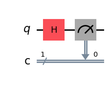
Build a simple circuit. Here we build one consisting of a single Hadamard gate on qubit \(0\), followed by measurement.
from qiskit import QuantumCircuit

circ = QuantumCircuit(1, 1)
circ.h(0)
circ.measure([0], [0])

circ.draw("mpl")
Next, attach a calibration for the Hadamard gate on qubit \(0\) to the circuit. Note that here we are only demonstrating the mechanics of adding a calibration; we have not attempted to calibrate the schedule to implement the Hadamard gate with high fidelity.
with pulse.build() as h_q0:
    pulse.play(
        pulse.library.Gaussian(duration=256, amp=0.2, sigma=50, name="custom"),
        pulse.DriveChannel(0)
    )

circ.add_calibration("h", qubits=[0], schedule=h_q0)
Call run on the circuit, and get counts as usual.
%time res = backend.run(circ).result()

res.get_counts(0)
CPU times: user 650 ms, sys: 123 ms, total: 773 ms
Wall time: 685 ms
{'0': 756, '1': 268}
4.2 Simulating circuits via gate definitions in the backend Target#
Alternatively to the above work flow, add the above schedule as the pulse-level definition of the
Hadamard gate on qubit \(0\) to backend.target, which impacts how jobs are transpiled for the
backend. See the Target class documentation for further information.
from qiskit.circuit.library import HGate
from qiskit.transpiler import InstructionProperties

backend.target.add_instruction(HGate(), {(0,): InstructionProperties(calibration=h_q0)})
Rebuild the same circuit, however this time we do not need to add the calibration for the Hadamard gate to the circuit object.
circ2 = QuantumCircuit(1, 1)
circ2.h(0)
circ2.measure([0], [0])

%time result = backend.run(circ2).result()
CPU times: user 753 ms, sys: 29.2 ms, total: 783 ms
Wall time: 777 ms
result.get_counts(0)
{'0': 778, '1': 246}
5. Simulating single-qubit calibration processes via Qiskit Experiments#
Next, we perform rough calibrations for X and SX gates on both qubits modeled in the
DynamicsBackend, following the single-qubit calibration tutorial for Qiskit Experiments.
5.1 Configure the Target to include single qubit instructions#
To enable running of the single qubit experiments, we add the following to the target:
Qubit frequency properties (needed by experiments like
RoughFrequencyCal). Note that setting the qubit frequencies in thetargetdoes not impact the behaviour of theDynamicsBackenditself. It is purely a data field that does not impact functionality. Previously set frequency properties, such aschannel_carrier_freqsin theSolver, will remain unchanged. Here, we set the frequencies to the undressed frequencies in the model.XandSXgate instructions, which the transpiler needs to check are supported by the backend.Add definitions of
RZgates as phase shifts. These instructions control the phase of the drive channels, as well as any control channels acting on a given qubit.Add a
CXgate between qubits \((0, 1)\) and \((1, 0)\). While this tutorial will not be utilizing it, this ensures that validation steps checking that the device is fully connected will pass.
from qiskit.circuit.library import XGate, SXGate, RZGate, CXGate
from qiskit.circuit import Parameter
from qiskit.providers.backend import QubitProperties

target = backend.target

# qubit properties
target.qubit_properties = [QubitProperties(frequency=v0), QubitProperties(frequency=v1)]

# add instructions
target.add_instruction(XGate(), properties={(0,): None, (1,): None})
target.add_instruction(SXGate(), properties={(0,): None, (1,): None})

target.add_instruction(CXGate(), properties={(0, 1): None, (1, 0): None})

# Add RZ instruction as phase shift for drag cal
phi = Parameter("phi")
with pulse.build() as rz0:
    pulse.shift_phase(phi, pulse.DriveChannel(0))
    pulse.shift_phase(phi, pulse.ControlChannel(1))

with pulse.build() as rz1:
    pulse.shift_phase(phi, pulse.DriveChannel(1))
    pulse.shift_phase(phi, pulse.ControlChannel(0))

target.add_instruction(
    RZGate(phi),
    {(0,): InstructionProperties(calibration=rz0), (1,): InstructionProperties(calibration=rz1)}
)
5.2 Prepare Calibrations object#
Next, prepare the Calibrations
object. Here we use the
FixedFrequencyTransmon
template library to initialize our calibrations.
import pandas as pd
from qiskit_experiments.calibration_management.calibrations import Calibrations
from qiskit_experiments.calibration_management.basis_gate_library import FixedFrequencyTransmon

cals = Calibrations(libraries=[FixedFrequencyTransmon(basis_gates=['x', 'sx'])])

pd.DataFrame(**cals.parameters_table(qubit_list=[0, ()]))
| parameter | qubits | schedule | value | group | valid | date_time | exp_id | |
|---|---|---|---|---|---|---|---|---|
| 0 | angle | () | sx | 0.00 | default | True | 2024-03-25 17:18:12.439070+0000 | None |
| 1 | angle | () | x | 0.00 | default | True | 2024-03-25 17:18:12.439034+0000 | None |
| 2 | β | () | x | 0.00 | default | True | 2024-03-25 17:18:12.438994+0000 | None |
| 3 | β | () | sx | 0.00 | default | True | 2024-03-25 17:18:12.439082+0000 | None |
| 4 | amp | () | sx | 0.25 | default | True | 2024-03-25 17:18:12.439060+0000 | None |
| 5 | amp | () | x | 0.50 | default | True | 2024-03-25 17:18:12.439026+0000 | None |
| 6 | duration | () | sx | 160.00 | default | True | 2024-03-25 17:18:12.439052+0000 | None |
| 7 | duration | () | x | 160.00 | default | True | 2024-03-25 17:18:12.439017+0000 | None |
| 8 | σ | () | sx | 40.00 | default | True | 2024-03-25 17:18:12.439089+0000 | None |
| 9 | σ | () | x | 40.00 | default | True | 2024-03-25 17:18:12.439041+0000 | None |
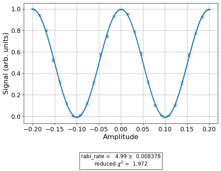
5.3 Rough amplitude calibration#
Next, run a rough amplitude calibration for X and SX gates for both qubits. First, build the
experiments.
from qiskit_experiments.library.calibration import RoughXSXAmplitudeCal

# rabi experiments for qubit 0
rabi0 = RoughXSXAmplitudeCal([0], cals, backend=backend, amplitudes=np.linspace(-0.2, 0.2, 27))

# rabi experiments for qubit 1
rabi1 = RoughXSXAmplitudeCal([1], cals, backend=backend, amplitudes=np.linspace(-0.2, 0.2, 27))
Run the Rabi experiments.
%%time
rabi0_data = rabi0.run().block_for_results()
rabi1_data = rabi1.run().block_for_results()
CPU times: user 5.44 s, sys: 774 ms, total: 6.22 s
Wall time: 5.53 s
Plot the results.
rabi0_data.figure(0)
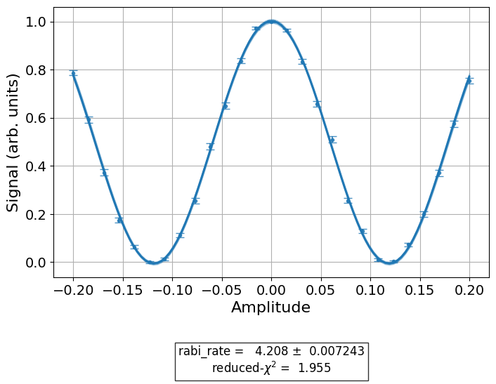
rabi1_data.figure(0)
Observe the updated parameters for qubit 0.
pd.DataFrame(**cals.parameters_table(qubit_list=[0, ()], parameters="amp"))
| parameter | qubits | schedule | value | group | valid | date_time | exp_id | |
|---|---|---|---|---|---|---|---|---|
| 0 | amp | () | x | 0.500000 | default | True | 2024-03-25 17:18:12.439026+0000 | None |
| 1 | amp | (0,) | sx | 0.059405 | default | True | 2024-03-25 17:18:13.441005+0000 | 50f54a2d-57de-4b9c-b152-9e037c574854 |
| 2 | amp | (0,) | x | 0.118810 | default | True | 2024-03-25 17:18:13.441005+0000 | 50f54a2d-57de-4b9c-b152-9e037c574854 |
| 3 | amp | () | sx | 0.250000 | default | True | 2024-03-25 17:18:12.439060+0000 | None |
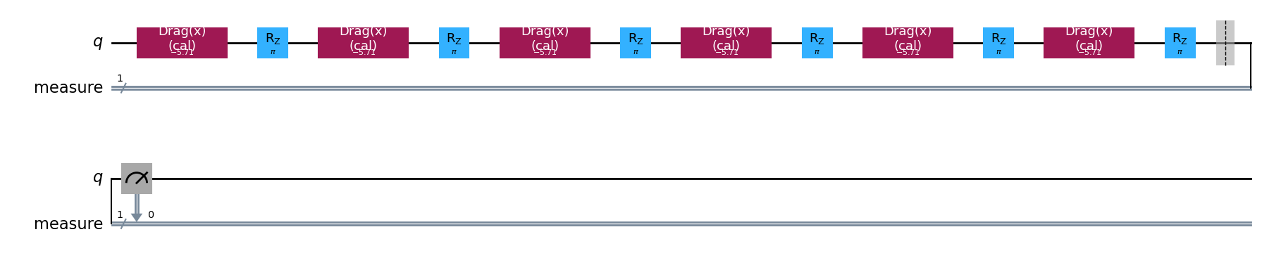
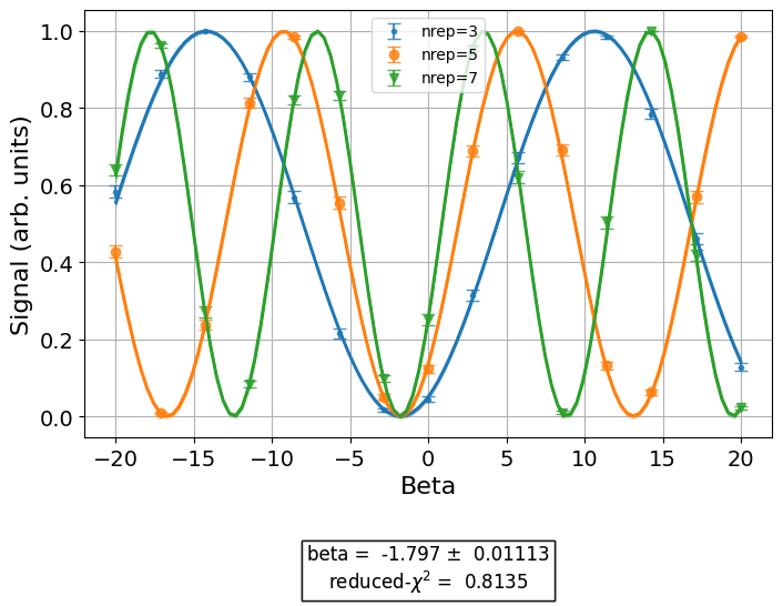
5.4 Rough Drag parameter calibration#
Run rough Drag parameter calibration for the X and SX gates. This follows the same procedure
as above.
from qiskit_experiments.library.calibration import RoughDragCal

cal_drag0 = RoughDragCal([0], cals, backend=backend, betas=np.linspace(-20, 20, 15))
cal_drag1 = RoughDragCal([1], cals, backend=backend, betas=np.linspace(-20, 20, 15))

cal_drag0.set_experiment_options(reps=[3, 5, 7])
cal_drag1.set_experiment_options(reps=[3, 5, 7])

cal_drag0.circuits()[5].draw(output="mpl")
%%time
drag0_data = cal_drag0.run().block_for_results()
drag1_data = cal_drag1.run().block_for_results()
CPU times: user 20.9 s, sys: 15.9 s, total: 36.7 s
Wall time: 17.8 s
drag0_data.figure(0)

drag1_data.figure(0)
The updated calibrations object:
pd.DataFrame(**cals.parameters_table(qubit_list=[0, ()], parameters="amp"))
| parameter | qubits | schedule | value | group | valid | date_time | exp_id | |
|---|---|---|---|---|---|---|---|---|
| 0 | amp | () | x | 0.500000 | default | True | 2024-03-25 17:18:12.439026+0000 | None |
| 1 | amp | (0,) | sx | 0.059405 | default | True | 2024-03-25 17:18:13.441005+0000 | 50f54a2d-57de-4b9c-b152-9e037c574854 |
| 2 | amp | (0,) | x | 0.118810 | default | True | 2024-03-25 17:18:13.441005+0000 | 50f54a2d-57de-4b9c-b152-9e037c574854 |
| 3 | amp | () | sx | 0.250000 | default | True | 2024-03-25 17:18:12.439060+0000 | None |
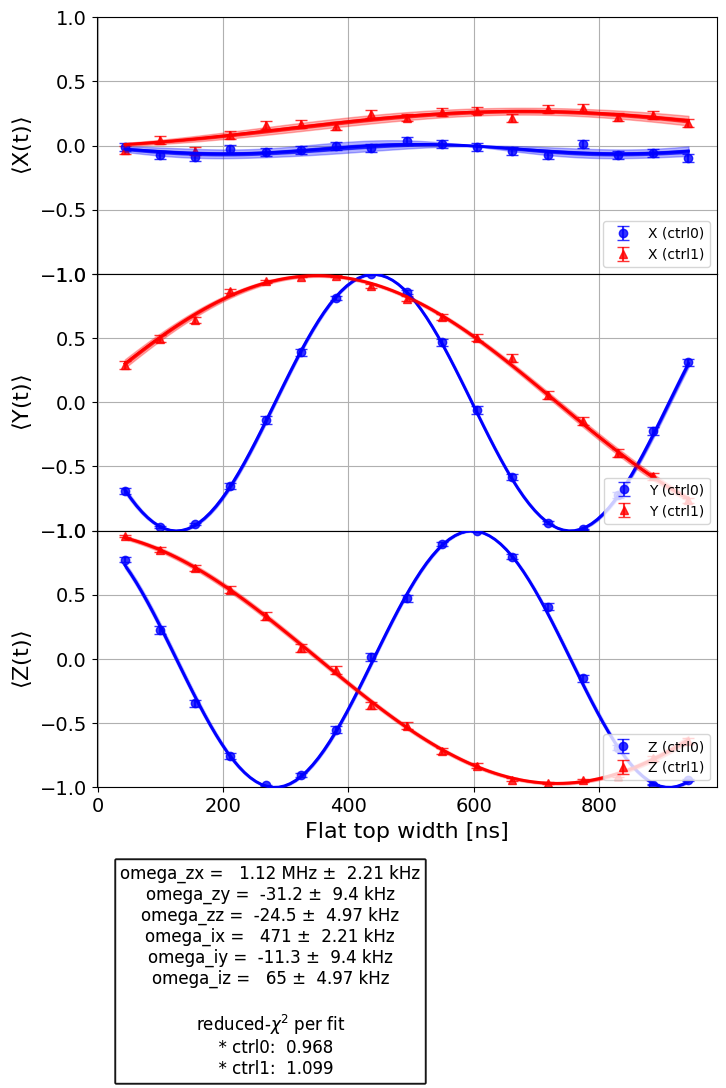
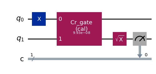
6. Simulating 2 qubit interaction characterization via the CrossResonanceHamiltonian experiment#
Finally, simulate the CrossResonanceHamiltonian characterization experiment.
First, we further configure the backend to run this experiment. This requires defining the control channel map, which is a dictionary mapping control-target qubit index pairs (given as a tuple) to the control channel index used to drive the corresponding cross-resonance interaction. This is required by the experiment to determine which channel to drive for each control-target pair.
# set the control channel map
backend.set_options(control_channel_map={(0, 1): 0, (1, 0): 1})
Build the characterization experiment object, and update gate definitions in target with the
values for the single qubit gates calibrated above.
from qiskit_experiments.library import CrossResonanceHamiltonian

cr_ham_experiment = CrossResonanceHamiltonian(
    physical_qubits=(0, 1),
    durations=np.linspace(1e-7, 1e-6, 17),
    backend=backend
)

backend.target.update_from_instruction_schedule_map(cals.get_inst_map())
cr_ham_experiment.circuits()[10].draw("mpl")
Run the simulation.
%time data_cr = cr_ham_experiment.run().block_for_results()
CPU times: user 17 s, sys: 5.29 s, total: 22.3 s
Wall time: 17 s
data_cr.figure(0)