Simulating Qiskit Pulse Schedules with Qiskit Dynamics#
This tutorial shows how to use Qiskit Dynamics to simulate a Pulse schedule with a simple model of a qubit. The qubit is modeled by the drift hamiltonian
to which we apply the drive
Here, \(\Omega(t)\) is the drive signal which we will create using Qiskit pulse. The factor
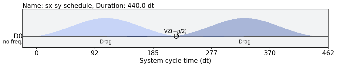
\(r\) is the strength with which the drive signal drives the qubit. We begin by creating a pulse
schedule with a sx gate followed by a phase shift on the drive so that the following pulse
creates a sy rotation. Therefore, if the qubit begins in the ground state we expect that this
second pulse will not have any effect on the qubit. This situation is simulated with the following
steps:
Create the pulse schedule.
Converting pulse schedules to a
Signal.Create the system model, configured to simulate pulse schedules.
Simulate the pulse schedule using the model.
1. Create the pulse schedule#
First, we use the pulse module in Qiskit to create a pulse schedule.
import numpy as np
import qiskit.pulse as pulse

# Strength of the Rabi-rate in GHz.
r = 0.1

# Frequency of the qubit transition in GHz.
w = 5.

# Sample rate of the backend in ns.
dt = 1 / 4.5

# Define gaussian envelope function to approximately implement an sx gate.
amp = 1. / 1.75
sig = 0.6985/r/amp
T = 4*sig
duration = int(T / dt)
beta = 2.0

with pulse.build(name="sx-sy schedule") as sxp:
    pulse.play(pulse.Drag(duration, amp, sig / dt, beta), pulse.DriveChannel(0))
    pulse.shift_phase(np.pi/2, pulse.DriveChannel(0))
    pulse.play(pulse.Drag(duration, amp, sig / dt, beta), pulse.DriveChannel(0))

sxp.draw()
2. Convert the pulse schedule to a Signal#
Qiskit Dynamics has functionality for converting pulse schedule to instances of Signal.
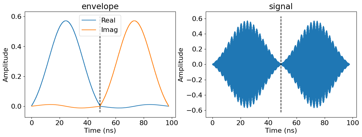
This is done using the pulse instruction to signal converter InstructionToSignals. This
converter needs to know the sample rate of the arbitrary waveform generators creating the signals,
i.e. dt, as well as the carrier frequency of the signals, i.e. w. The plot below shows the
envelopes and the signals resulting from this conversion. The dashed line shows the time at which
the virtual Z gate is applied.
from matplotlib import pyplot as plt
from qiskit_dynamics.pulse import InstructionToSignals

plt.rcParams["font.size"] = 16

converter = InstructionToSignals(dt, carriers={"d0": w})

signals = converter.get_signals(sxp)
fig, axs = plt.subplots(1, 2, figsize=(14, 4.5))
for ax, title in zip(axs, ["envelope", "signal"]):
    signals[0].draw(0, 2*T, 2000, title, axis=ax)
    ax.set_xlabel("Time (ns)")
    ax.set_ylabel("Amplitude")
    ax.set_title(title)
    ax.vlines(T, ax.get_ylim()[0], ax.get_ylim()[1], "k", linestyle="dashed")
3. Create the system model#
We now setup a Solver instance with the desired Hamiltonian information, and configure it
to simulate pulse schedules. This requires specifying which channels act on which operators, channel
carrier frequencies, and sample width dt. Additionally, we setup this solver in the rotating
frame and perform the rotating wave approximation.
from qiskit.quantum_info.operators import Operator
from qiskit_dynamics import Solver

# construct operators
X = Operator.from_label('X')
Z = Operator.from_label('Z')

drift = 2 * np.pi * w * Z/2
operators = [2 * np.pi * r * X/2]

# construct the solver
hamiltonian_solver = Solver(
    static_hamiltonian=drift,
    hamiltonian_operators=operators,
    rotating_frame=drift,
    rwa_cutoff_freq=2 * 5.0,
    hamiltonian_channels=['d0'],
    channel_carrier_freqs={'d0': w},
    dt=dt
)
4. Simulate the pulse schedule using the model#
In the last step we perform the simulation and plot the results. Note that, as we have configured
hamiltonian_solver to simulate pulse schedules, we pass the schedule xp directly to the
signals argument of the solve method. Equivalently, signals generated by
converter.get_signals above can also be passed to the signals argument and in this case
should produce identical behavior.
from qiskit.quantum_info.states import Statevector

# Start the qubit in its ground state.
y0 = Statevector([1., 0.])

%time sol = hamiltonian_solver.solve(t_span=[0., 2*T], y0=y0, signals=sxp, atol=1e-8, rtol=1e-8)
CPU times: user 15.3 s, sys: 6.9 ms, total: 15.3 s
Wall time: 15.3 s
def plot_populations(sol):
    pop0 = [psi.probabilities()[0] for psi in sol.y]
    pop1 = [psi.probabilities()[1] for psi in sol.y]

    fig = plt.figure(figsize=(8, 5))
    plt.plot(sol.t, pop0, lw=3, label="Population in |0>")
    plt.plot(sol.t, pop1, lw=3, label="Population in |1>")
    plt.xlabel("Time (ns)")
    plt.ylabel("Population")
    plt.legend(frameon=False)
    plt.ylim([0, 1.05])
    plt.xlim([0, 2*T])
    plt.vlines(T, 0, 1.05, "k", linestyle="dashed")
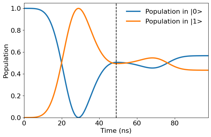
The plot below shows the population of the qubit as it evolves during the pulses. The vertical
dashed line shows the time of the virtual Z rotation which was induced by the shift_phase
instruction in the pulse schedule. As expected, the first pulse moves the qubit to an eigenstate of
the Y operator. Therefore, the second pulse, which drives around the Y-axis due to the phase
shift, has hardley any influence on the populations of the qubit.
plot_populations(sol)