Note

This page was generated from docs/tutorials/06_grover.ipynb.

Grover’s Algorithm and Amplitude Amplification

Grover’s algorithm is one of the most famous quantum algorithms introduced by Lov Grover in 1996 [1]. It has initially been proposed for unstructured search problems, i.e. for finding a marked element in a unstructured database. However, Grover’s algorithm is now a subroutine to several other algorithms, such as Grover Adaptive Search [2]. For the details of Grover’s algorithm, please see Grover’s Algorithm in the Qiskit textbook.

Qiskit implements Grover’s algorithm in the Grover class. This class also includes the generalized version, Amplitude Amplification [3], and allows setting individual iterations and other meta-settings to Grover’s algorithm.

References:

[1]: L. K. Grover, A fast quantum mechanical algorithm for database search. Proceedings 28th Annual Symposium on the Theory of Computing (STOC) 1996, pp. 212-219. https://arxiv.org/abs/quant-ph/9605043

[2]: A. Gilliam, S. Woerner, C. Gonciulea, Grover Adaptive Search for Constrained Polynomial Binary Optimization. https://arxiv.org/abs/1912.04088

[3]: Brassard, G., Hoyer, P., Mosca, M., & Tapp, A. (2000). Quantum Amplitude Amplification and Estimation. http://arxiv.org/abs/quant-ph/0005055

Grover’s algorithm

Grover’s algorithm uses the Grover operator \(\mathcal{Q}\) to amplify the amplitudes of the good states:

\[\mathcal{Q} = \mathcal{A}\mathcal{S_0}\mathcal{A}^\dagger \mathcal{S_f}\]

Here, * \(\mathcal{A}\) is the initial search state for the algorithm, which is just Hadamards, \(H^{\otimes n}\) for the textbook Grover search, but can be more elaborate for Amplitude Amplification * \(\mathcal{S_0}\) is the reflection about the all 0 state

\[\begin{split}|x\rangle \mapsto \begin{cases} -|x\rangle, &x \neq 0 \\ |x\rangle, &x = 0\end{cases}\end{split}\]

* \(\mathcal{S_f}\) is the oracle that applies

\[|x\rangle \mapsto (-1)^{f(x)}|x\rangle\]

    　where \(f(x)\) is 1 if \(x\) is a good state and otherwise 0.

In a nutshell, Grover’s algorithm applies different powers of \(\mathcal{Q}\) and after each execution checks whether a good solution has been found.

Running Grover’s algorithm

To run Grover’s algorithm with the Grover class, firstly, we need to specify an oracle for the circuit of Grover’s algorithm. In the following example, we use QuantumCircuit as the oracle of Grover’s algorithm. However, there are several other class that we can use as the oracle of Grover’s algorithm. We talk about them later in this tutorial.

Note that the oracle for Grover must be a phase-flip oracle. That is, it multiplies the amplitudes of the of “good states” by a factor of \(-1\). We explain later how to convert a bit-flip oracle to a phase-flip oracle.

from qiskit import QuantumCircuit
from qiskit_algorithms import AmplificationProblem

# the state we desire to find is '11'
good_state = ["11"]

# specify the oracle that marks the state '11' as a good solution
oracle = QuantumCircuit(2)
oracle.cz(0, 1)

# define Grover's algorithm
problem = AmplificationProblem(oracle, is_good_state=good_state)

# now we can have a look at the Grover operator that is used in running the algorithm
# (Algorithm circuits are wrapped in a gate to appear in composition as a block
# so we have to decompose() the op to see it expanded into its component gates.)
problem.grover_operator.decompose().draw(output="mpl")

Then, we specify a backend and call the run method of Grover with a backend to execute the circuits. The returned result type is a GroverResult.

If the search was successful, the oracle_evaluation attribute of the result will be True. In this case, the most sampled measurement, top_measurement, is one of the “good states”. Otherwise, oracle_evaluation will be False.

from qiskit_algorithms import Grover
from qiskit.primitives import Sampler


grover = Grover(sampler=Sampler())
result = grover.amplify(problem)
print("Result type:", type(result))
print()
print("Success!" if result.oracle_evaluation else "Failure!")
print("Top measurement:", result.top_measurement)

Result type: <class 'qiskit_algorithms.amplitude_amplifiers.grover.GroverResult'>

Success!
Top measurement: 11

In the example, the result of top_measurement is 11 which is one of “good state”. Thus, we succeeded to find the answer by using Grover.

Using the different types of classes as the oracle of Grover

In the above example, we used QuantumCircuit as the oracle of Grover. However, we can also use qiskit.quantum_info.Statevector as oracle. All the following examples are when \(|11\rangle\) is “good state”

from qiskit.quantum_info import Statevector

oracle = Statevector.from_label("11")
problem = AmplificationProblem(oracle, is_good_state=["11"])

grover = Grover(sampler=Sampler())
result = grover.amplify(problem)
print("Result type:", type(result))
print()
print("Success!" if result.oracle_evaluation else "Failure!")
print("Top measurement:", result.top_measurement)

Result type: <class 'qiskit_algorithms.amplitude_amplifiers.grover.GroverResult'>

Success!
Top measurement: 11

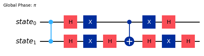
Internally, the statevector is mapped to a quantum circuit:

problem.grover_operator.oracle.decompose().draw(output="mpl")

Qiskit allows for an easy construction of more complex oracles: * PhaseOracle: for parsing logical expressions such as '~a | b'. This is especially useful for solving 3-SAT problems and is shown in the accompanying Grover Examples tutorial.

Here we’ll use the PhaseOracle for the simple example of finding the state \(|11\rangle\), which corresponds to 'a & b'.

from qiskit.circuit.library.phase_oracle import PhaseOracle
from qiskit.exceptions import MissingOptionalLibraryError

# `Oracle` (`PhaseOracle`) as the `oracle` argument
expression = "(a & b)"
try:
    oracle = PhaseOracle(expression)
    problem = AmplificationProblem(oracle)
    display(problem.grover_operator.oracle.decompose().draw(output="mpl"))
except MissingOptionalLibraryError as ex:
    print(ex)

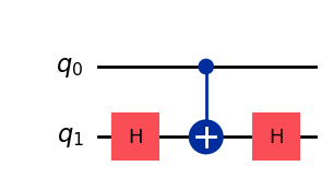
Which we observe that this oracle implements a phase flip when the state is \(|11\rangle\)

As mentioned above, Grover’s algorithm requires a phase-flip oracle. A bit-flip oracle flips the state of an auxiliary qubit if the other qubits satisfy the condition. To use these types of oracles with Grover’s we need to convert the bit-flip oracle to a phase-flip oracle by sandwiching the auxiliary qubit of the bit-flip oracle by \(X\) and \(H\) gates.

Note: This transformation from a bit-flip to a phase-flip oracle holds generally and you can use this to convert your oracle to the right representation.

Amplitude amplification

Grover’s algorithm uses Hadamard gates to create the uniform superposition of all the states at the beginning of the Grover operator \(\mathcal{Q}\). If some information on the good states is available, it might be useful to not start in a uniform superposition but only initialize specific states. This, generalized, version of Grover’s algorithm is referred to Amplitude Amplification.

In Qiskit, the initial superposition state can easily be adjusted by setting the state_preparation argument.

State preparation

A state_preparation argument is used to specify a quantum circuit that prepares a quantum state for the start point of the amplitude amplification. By default, a circuit with \(H^{\otimes n}\) is used to prepare uniform superposition (so it will be Grover’s search). The diffusion circuit of the amplitude amplification reflects state_preparation automatically.

import numpy as np

# Specifying `state_preparation`
# to prepare a superposition of |01>, |10>, and |11>
oracle = QuantumCircuit(3)
oracle.ccz(0, 1, 2)

theta = 2 * np.arccos(1 / np.sqrt(3))
state_preparation = QuantumCircuit(3)
state_preparation.ry(theta, 0)
state_preparation.ch(0, 1)
state_preparation.x(1)
state_preparation.h(2)

# we only care about the first two bits being in state 1, thus add both possibilities for the last qubit
problem = AmplificationProblem(
    oracle, state_preparation=state_preparation, is_good_state=["110", "111"]
)

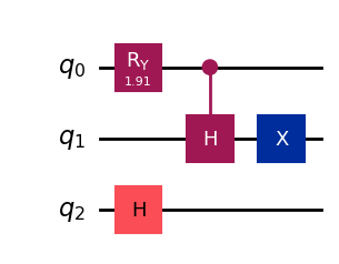
# state_preparation
print("state preparation circuit:")
problem.grover_operator.state_preparation.draw(output="mpl")

state preparation circuit:

grover = Grover(sampler=Sampler())
result = grover.amplify(problem)
print("Success!" if result.oracle_evaluation else "Failure!")
print("Top measurement:", result.top_measurement)

Success!
Top measurement: 111

Full flexibility

For more advanced use, it is also possible to specify the entire Grover operator by setting the grover_operator argument. This might be useful if you know more efficient implementation for \(\mathcal{Q}\) than the default construction via zero reflection, oracle and state preparation.

The qiskit.circuit.library.GroverOperator can be a good starting point and offers more options for an automated construction of the Grover operator. You can for instance * set the mcx_mode * ignore qubits in the zero reflection by setting reflection_qubits * explicitly exchange the \(\mathcal{S_f}, \mathcal{S_0}\) and \(\mathcal{A}\) operations using the oracle, zero_reflection and state_preparation arguments

For instance, imagine the good state is a three qubit state \(|111\rangle\) but we used 2 additional qubits as auxiliary qubits.

oracle = QuantumCircuit(5)
oracle.ccz(0, 1, 2)
oracle.draw(output="mpl")

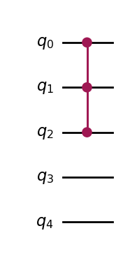
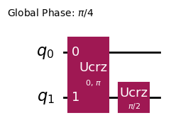
Then, per default, the Grover operator implements the zero reflection on all five qubits.

from qiskit.circuit.library import GroverOperator

grover_op = GroverOperator(oracle, insert_barriers=True)
grover_op.decompose().draw(output="mpl")

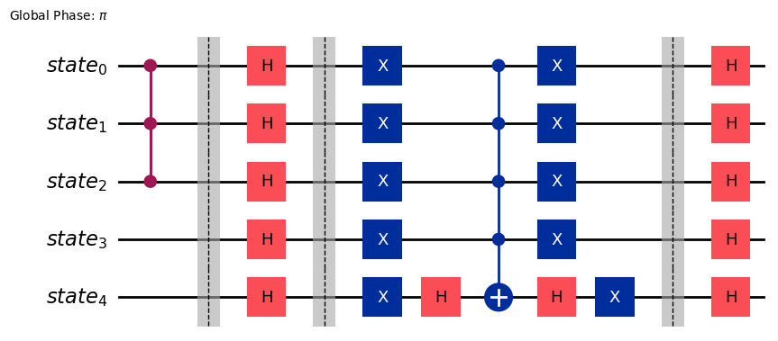
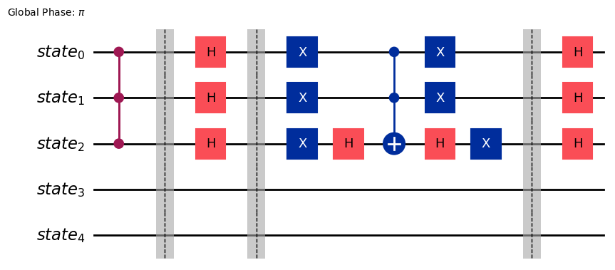
But we know that we only need to consider the first three:

grover_op = GroverOperator(oracle, reflection_qubits=[0, 1, 2], insert_barriers=True)
grover_op.decompose().draw(output="mpl")

Dive into other arguments of Grover

Grover has arguments other than oracle and state_preparation. We will explain them in this section.

Specifying good_state

good_state is used to check whether the measurement result is correct or not internally. It can be a list of binary strings, a list of integer, Statevector, and Callable. If the input is a list of bitstrings, each bitstrings in the list represents a good state. If the input is a list of integer, each integer represent the index of the good state to be \(|1\rangle\). If it is a Statevector, it represents a superposition of all good states.

# a list of binary strings good state
oracle = QuantumCircuit(2)
oracle.cz(0, 1)
good_state = ["11", "00"]
problem = AmplificationProblem(oracle, is_good_state=good_state)
print(problem.is_good_state("11"))

True

# a list of integer good state
oracle = QuantumCircuit(2)
oracle.cz(0, 1)
good_state = [0, 1]
problem = AmplificationProblem(oracle, is_good_state=good_state)
print(problem.is_good_state("11"))

True

from qiskit.quantum_info import Statevector

# `Statevector` good state
oracle = QuantumCircuit(2)
oracle.cz(0, 1)
good_state = Statevector.from_label("11")
problem = AmplificationProblem(oracle, is_good_state=good_state)
print(problem.is_good_state("11"))

True

# Callable good state
def callable_good_state(bitstr):
    if bitstr == "11":
        return True
    return False


oracle = QuantumCircuit(2)
oracle.cz(0, 1)
problem = AmplificationProblem(oracle, is_good_state=good_state)
print(problem.is_good_state("11"))

True

The number of iterations

The number of repetition of applying the Grover operator is important to obtain the correct result with Grover’s algorithm. The number of iteration can be set by the iteration argument of Grover. The following inputs are supported: * an integer to specify a single power of the Grover operator that’s applied * or a list of integers, in which all these different powers of the Grover operator are run consecutively and after each time we check if a correct solution has been found

Additionally there is the sample_from_iterations argument. When it is True, instead of the specific power in iterations, a random integer between 0 and the value in iteration is used as the power Grover’s operator. This approach is useful when we don’t even know the number of solution.

For more details of the algorithm using sample_from_iterations, see [4].

References:

[4]: Boyer et al., Tight bounds on quantum searching arxiv:quant-ph/9605034

# integer iteration
oracle = QuantumCircuit(2)
oracle.cz(0, 1)
problem = AmplificationProblem(oracle, is_good_state=["11"])
grover = Grover(iterations=1)

# list iteration
oracle = QuantumCircuit(2)
oracle.cz(0, 1)
problem = AmplificationProblem(oracle, is_good_state=["11"])
grover = Grover(iterations=[1, 2, 3])

# using sample_from_iterations
oracle = QuantumCircuit(2)
oracle.cz(0, 1)
problem = AmplificationProblem(oracle, is_good_state=["11"])
grover = Grover(iterations=[1, 2, 3], sample_from_iterations=True)

When the number of solutions is known, we can also use a static method optimal_num_iterations to find the optimal number of iterations. Note that the output iterations is an approximate value. When the number of qubits is small, the output iterations may not be optimal. In addition, the calculation of this value assumes the standard uniform superposition state preparation and may not be accurate for other state preparations.

iterations = Grover.optimal_num_iterations(num_solutions=1, num_qubits=8)
iterations

12

Applying post_processing

We can apply an optional post processing to the top measurement for ease of readability. It can be used e.g. to convert from the bit-representation of the measurement [1, 0, 1] to a DIMACS CNF format [1, -2, 3].

def to_DIAMACS_CNF_format(bit_rep):
    return [index + 1 if val == 1 else -1 * (index + 1) for index, val in enumerate(bit_rep)]


oracle = QuantumCircuit(2)
oracle.cz(0, 1)
problem = AmplificationProblem(oracle, is_good_state=["11"], post_processing=to_DIAMACS_CNF_format)
problem.post_processing([1, 0, 1])

[1, -2, 3]

import tutorial_magics

%qiskit_version_table
%qiskit_copyright

Version Information

Software	Version
qiskit	1.0.2
qiskit_algorithms	0.3.0
System information
Python version	3.8.18
OS	Linux
Wed Apr 10 17:19:01 2024 UTC

This code is a part of a Qiskit project

© Copyright IBM 2017, 2024.

This code is licensed under the Apache License, Version 2.0. You may
obtain a copy of this license in the LICENSE.txt file in the root directory
of this source tree or at http://www.apache.org/licenses/LICENSE-2.0.

Any modifications or derivative works of this code must retain this
copyright notice, and modified files need to carry a notice indicating
that they have been altered from the originals.