Note

This page was generated from docs/tutorials/04_vqd.ipynb.

Variational Quantum Deflation (VQD) Algorithm

This notebook demonstrates how to use our implementation of the Variational Quantum Deflation (VQD) algorithm for computing higher energy states of a Hamiltonian, as introduced in this reference paper.

Introduction

VQD is a quantum algorithm that uses a variational technique to find the k eigenvalues of the Hamiltonian H of a given system.

The algorithm computes excited state energies of generalized hamiltonians by optimizing over a modified cost function. Each successive eigenvalue is calculated iteratively by introducing an overlap term with all the previously computed eigenstates that must be minimized. This ensures that higher energy eigenstates are found.

Complete working example for VQD

The first step of the VQD workflow is to create a qubit operator, ansatz and optimizer. For this example, you can use the H2 molecule, which should already look familiar if you have completed the previous VQE tutorials:

from qiskit.quantum_info import SparsePauliOp

H2_op = SparsePauliOp.from_list(
    [
        ("II", -1.052373245772859),
        ("IZ", 0.39793742484318045),
        ("ZI", -0.39793742484318045),
        ("ZZ", -0.01128010425623538),
        ("XX", 0.18093119978423156),
    ]
)

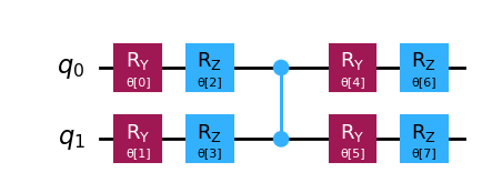
You can set up, for example, a TwoLocal ansatz with two qubits, and choose SLSQP as the optimization method.

from qiskit.circuit.library import TwoLocal
from qiskit_algorithms.optimizers import SLSQP

ansatz = TwoLocal(2, rotation_blocks=["ry", "rz"], entanglement_blocks="cz", reps=1)

optimizer = SLSQP()
ansatz.decompose().draw("mpl")

The next step of the workflow is to define the required primitives for running VQD. This algorithm requires two different primitive instances: one Estimator for computing the expectation values for the “VQE part” of the algorithm, and one Sampler. The sampler will be passed along to the StateFidelity subroutine that will be used to compute the cost for higher energy states. There are several methods that you can use to compute state fidelities, but to keep things simple, you can use the ComputeUncompute method already available in qiskit_algorithm.state_fidelities.

from qiskit.primitives import Sampler, Estimator
from qiskit_algorithms.state_fidelities import ComputeUncompute

estimator = Estimator()
sampler = Sampler()
fidelity = ComputeUncompute(sampler)

In order to set up the VQD algorithm, it is important to define two additional inputs: the number of energy states to compute (k) and the betas defined in the original VQD paper. In this example, the number of states (k) will be set to three, which indicates that two excited states will be computed in addition to the ground state.

The betas balance the contribution of each overlap term to the cost function, and they are an optional argument in the VQD construction. If not set by the user, they can be auto-evaluated for input operators of type SparsePauliOp. Please note that if you want to set your own betas, you should provide a list of values of length k.

k = 3
betas = [33, 33, 33]

You are almost ready to run the VQD algorithm, but let’s define a callback first to store intermediate values:

counts = []
values = []
steps = []


def callback(eval_count, params, value, meta, step):
    counts.append(eval_count)
    values.append(value)
    steps.append(step)

You can finally instantiate VQD and compute the eigenvalues for the chosen operator.

from qiskit_algorithms import VQD

vqd = VQD(estimator, fidelity, ansatz, optimizer, k=k, betas=betas, callback=callback)
result = vqd.compute_eigenvalues(operator=H2_op)
vqd_values = result.eigenvalues

You can see the three state energies as part of the VQD result:

print(vqd_values.real)

[-1.85720407 -1.24461715 -0.88274845]

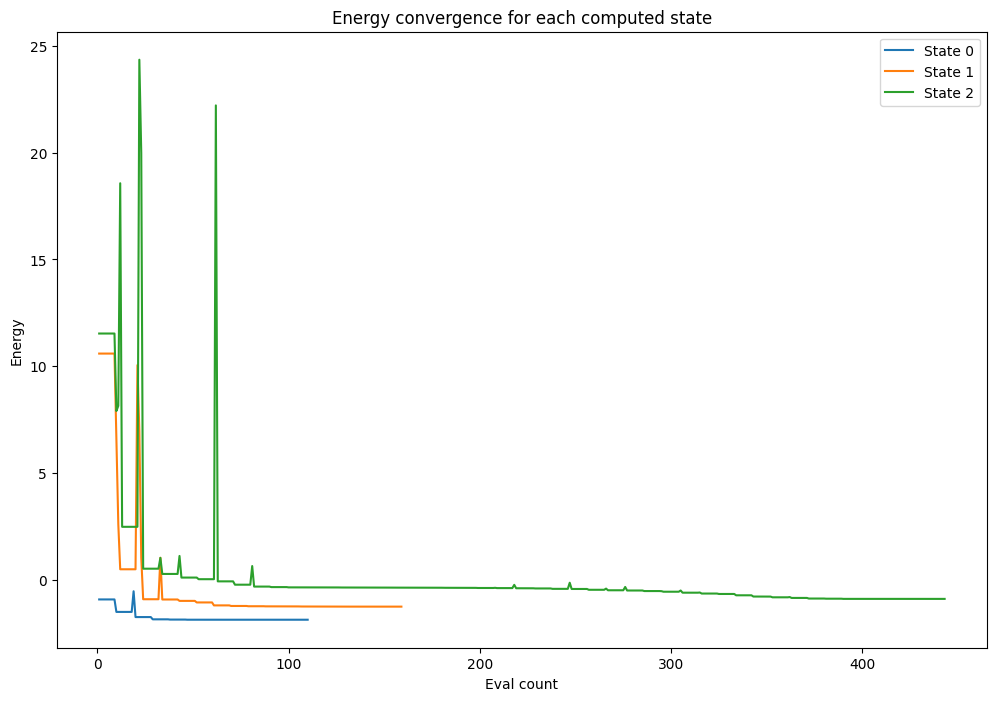
And we can use the values stored by the callback to plot the energy convergence for each state:

import numpy as np
import pylab

pylab.rcParams["figure.figsize"] = (12, 8)

steps = np.asarray(steps)
counts = np.asarray(counts)
values = np.asarray(values)

for i in range(1, 4):
    _counts = counts[np.where(steps == i)]
    _values = values[np.where(steps == i)]
    pylab.plot(_counts, _values, label=f"State {i-1}")

pylab.xlabel("Eval count")
pylab.ylabel("Energy")
pylab.title("Energy convergence for each computed state")
pylab.legend(loc="upper right");

This molecule can be solved exactly using the NumPyEigensolver class, which will give a reference value that you can compare with the VQD result:

from qiskit_algorithms import NumPyEigensolver


exact_solver = NumPyEigensolver(k=3)
exact_result = exact_solver.compute_eigenvalues(H2_op)
ref_values = exact_result.eigenvalues

Let’s see a comparison of the exact result with the previously computed VQD eigenvalues:

print(f"Reference values: {ref_values}")
print(f"VQD values: {vqd_values.real}")

Reference values: [-1.85727503 -1.24458455 -0.88272215]
VQD values: [-1.85720407 -1.24461715 -0.88274845]

As you can see, the result from VQD matches the values from the exact solution, and extends VQE to also compute excited states.

import tutorial_magics

%qiskit_version_table
%qiskit_copyright

Version Information

Software	Version
qiskit	1.0.2
qiskit_algorithms	0.3.0
System information
Python version	3.8.18
OS	Linux
Wed Apr 10 17:18:45 2024 UTC

This code is a part of a Qiskit project

© Copyright IBM 2017, 2024.

This code is licensed under the Apache License, Version 2.0. You may
obtain a copy of this license in the LICENSE.txt file in the root directory
of this source tree or at http://www.apache.org/licenses/LICENSE-2.0.

Any modifications or derivative works of this code must retain this
copyright notice, and modified files need to carry a notice indicating
that they have been altered from the originals.