Nota
Esta página fue generada a partir de docs/tutorials/10_lattice_models.ipynb.
Modelos de retícula#
Introducción#
En física cuántica (incluida la física de materia condensada y la física de altas energías), a menudo estudiamos modelos en retículas. Por ejemplo, cuando pensamos en el comportamiento de los electrones en un sólido, podemos estudiar un modelo definido en una malla considerando las posiciones de los átomos como puntos de la retícula. Este cuaderno demuestra cómo podemos utilizar las clases Lattice para generar varios sistemas de retícula como LineLattice, SquareLattice, HyperCubicLattice, TriangularLattice y una retícula general. También incluye un ejemplo de modelo de retícula, el modelo Fermi-Hubbard. Vemos cómo podemos definir el Hamiltoniano del modelo de Fermi-Hubbard para una retícula determinada usando la clase FermiHubbardModel.
[1]:
from math import pi

import numpy as np
import rustworkx as rx
from qiskit_nature.second_q.hamiltonians.lattices import (
    BoundaryCondition,
    HyperCubicLattice,
    Lattice,
    LatticeDrawStyle,
    LineLattice,
    SquareLattice,
    TriangularLattice,
)
from qiskit_nature.second_q.hamiltonians import FermiHubbardModel
LineLattice#
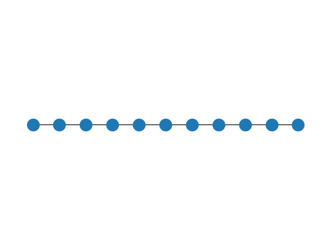
LineLattice proporciona una retícula unidimensional. Podemos construir una malla unidimensional de la siguiente manera.
[2]:
num_nodes = 11
boundary_condition = BoundaryCondition.OPEN
line_lattice = LineLattice(num_nodes=num_nodes, boundary_condition=boundary_condition)
Aquí se visualiza.
[3]:
line_lattice.draw()

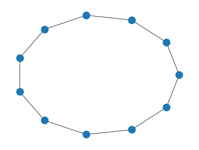
También podemos construir una retícula unidimensional con las condiciones de frontera periódicas especificando BoundaryCondition.PERIODIC como argumento de boundary_condition.
[4]:
num_nodes = 11
boundary_condition = BoundaryCondition.PERIODIC
line_lattice = LineLattice(num_nodes=num_nodes, boundary_condition=boundary_condition)

line_lattice.draw()
Cuando queremos dibujar la retícula ignorando las condiciones de frontera, usamos el método draw_without_boundary.
[5]:
line_lattice.draw_without_boundary()
Podemos definir pesos reales o complejos para los bordes de la retícula. Esto se hace dando un valor al argumento edge_parameter. También podemos dar un valor para los auto-bucles de la malla pasando el valor de onsite_parameter.
[6]:
num_nodes = 11
boundary_condition = BoundaryCondition.PERIODIC
edge_parameter = 1.0 + 1.0j
onsite_parameter = 1.0
line_lattice = LineLattice(
    num_nodes=num_nodes,
    edge_parameter=edge_parameter,
    onsite_parameter=onsite_parameter,
    boundary_condition=boundary_condition,
)
set(line_lattice.graph.weighted_edge_list())
[6]:
{(0, 0, 1.0),
 (0, 1, (1+1j)),
 (0, 10, (1-1j)),
 (1, 1, 1.0),
 (1, 2, (1+1j)),
 (2, 2, 1.0),
 (2, 3, (1+1j)),
 (3, 3, 1.0),
 (3, 4, (1+1j)),
 (4, 4, 1.0),
 (4, 5, (1+1j)),
 (5, 5, 1.0),
 (5, 6, (1+1j)),
 (6, 6, 1.0),
 (6, 7, (1+1j)),
 (7, 7, 1.0),
 (7, 8, (1+1j)),
 (8, 8, 1.0),
 (8, 9, (1+1j)),
 (9, 9, 1.0),
 (9, 10, (1+1j)),
 (10, 10, 1.0)}
La conectividad de la retícula se puede ver como la matriz de adyacencia, que se logra con to_adjacency_matrix.
[7]:
line_lattice.to_adjacency_matrix()
[7]:
array([[1., 1., 0., 0., 0., 0., 0., 0., 0., 0., 1.],
       [1., 1., 1., 0., 0., 0., 0., 0., 0., 0., 0.],
       [0., 1., 1., 1., 0., 0., 0., 0., 0., 0., 0.],
       [0., 0., 1., 1., 1., 0., 0., 0., 0., 0., 0.],
       [0., 0., 0., 1., 1., 1., 0., 0., 0., 0., 0.],
       [0., 0., 0., 0., 1., 1., 1., 0., 0., 0., 0.],
       [0., 0., 0., 0., 0., 1., 1., 1., 0., 0., 0.],
       [0., 0., 0., 0., 0., 0., 1., 1., 1., 0., 0.],
       [0., 0., 0., 0., 0., 0., 0., 1., 1., 1., 0.],
       [0., 0., 0., 0., 0., 0., 0., 0., 1., 1., 1.],
       [1., 0., 0., 0., 0., 0., 0., 0., 0., 1., 1.]])
Al establecer weighted=True, obtenemos una matriz Hermitiana cuyos elementos de matriz son los pesos.
[8]:
line_lattice.to_adjacency_matrix(weighted=True)
[8]:
array([[1.+0.j, 1.+1.j, 0.+0.j, 0.+0.j, 0.+0.j, 0.+0.j, 0.+0.j, 0.+0.j,
        0.+0.j, 0.+0.j, 1.-1.j],
       [1.-1.j, 1.+0.j, 1.+1.j, 0.+0.j, 0.+0.j, 0.+0.j, 0.+0.j, 0.+0.j,
        0.+0.j, 0.+0.j, 0.+0.j],
       [0.+0.j, 1.-1.j, 1.+0.j, 1.+1.j, 0.+0.j, 0.+0.j, 0.+0.j, 0.+0.j,
        0.+0.j, 0.+0.j, 0.+0.j],
       [0.+0.j, 0.+0.j, 1.-1.j, 1.+0.j, 1.+1.j, 0.+0.j, 0.+0.j, 0.+0.j,
        0.+0.j, 0.+0.j, 0.+0.j],
       [0.+0.j, 0.+0.j, 0.+0.j, 1.-1.j, 1.+0.j, 1.+1.j, 0.+0.j, 0.+0.j,
        0.+0.j, 0.+0.j, 0.+0.j],
       [0.+0.j, 0.+0.j, 0.+0.j, 0.+0.j, 1.-1.j, 1.+0.j, 1.+1.j, 0.+0.j,
        0.+0.j, 0.+0.j, 0.+0.j],
       [0.+0.j, 0.+0.j, 0.+0.j, 0.+0.j, 0.+0.j, 1.-1.j, 1.+0.j, 1.+1.j,
        0.+0.j, 0.+0.j, 0.+0.j],
       [0.+0.j, 0.+0.j, 0.+0.j, 0.+0.j, 0.+0.j, 0.+0.j, 1.-1.j, 1.+0.j,
        1.+1.j, 0.+0.j, 0.+0.j],
       [0.+0.j, 0.+0.j, 0.+0.j, 0.+0.j, 0.+0.j, 0.+0.j, 0.+0.j, 1.-1.j,
        1.+0.j, 1.+1.j, 0.+0.j],
       [0.+0.j, 0.+0.j, 0.+0.j, 0.+0.j, 0.+0.j, 0.+0.j, 0.+0.j, 0.+0.j,
        1.-1.j, 1.+0.j, 1.+1.j],
       [1.+1.j, 0.+0.j, 0.+0.j, 0.+0.j, 0.+0.j, 0.+0.j, 0.+0.j, 0.+0.j,
        0.+0.j, 1.-1.j, 1.+0.j]])
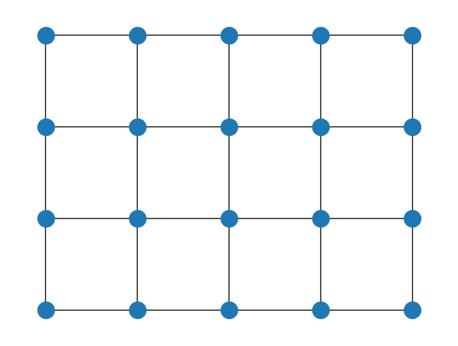
SquareLattice#
SquareLattice proporciona una retícula bidimensional. Aquí, hacemos una malla bidimensional con las condiciones de frontera abierta.
[9]:
rows = 5
cols = 4
boundary_condition = BoundaryCondition.OPEN
square_lattice = SquareLattice(rows=rows, cols=cols, boundary_condition=boundary_condition)

square_lattice.draw()
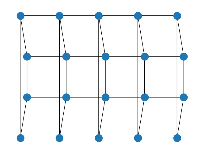
Podemos especificar las condiciones de frontera para cada dirección estableciendo boundary_condition como una tupla.
[10]:
rows = 5
cols = 4
boundary_condition = (
    BoundaryCondition.OPEN,
    BoundaryCondition.PERIODIC,
)  # open in the x-direction, periodic in the y-direction
square_lattice = SquareLattice(rows=rows, cols=cols, boundary_condition=boundary_condition)

square_lattice.draw()
Nuevamente, podemos dar pesos en los bordes y los auto-bucles de la retícula. Aquí, es posible dar pesos para cada dirección como una tupla.
[11]:
rows = 5
cols = 4
edge_parameter = (1.0, 1.0 + 1.0j)
boundary_condition = (
    BoundaryCondition.OPEN,
    BoundaryCondition.PERIODIC,
)  # open in the x-direction, periodic in the y-direction
onsite_parameter = 1.0
square_lattice = SquareLattice(
    rows=rows,
    cols=cols,
    edge_parameter=edge_parameter,
    onsite_parameter=onsite_parameter,
    boundary_condition=boundary_condition,
)

set(square_lattice.graph.weighted_edge_list())
[11]:
{(0, 0, 1.0),
 (0, 1, 1.0),
 (0, 5, (1+1j)),
 (0, 15, (1-1j)),
 (1, 1, 1.0),
 (1, 2, 1.0),
 (1, 6, (1+1j)),
 (1, 16, (1-1j)),
 (2, 2, 1.0),
 (2, 3, 1.0),
 (2, 7, (1+1j)),
 (2, 17, (1-1j)),
 (3, 3, 1.0),
 (3, 4, 1.0),
 (3, 8, (1+1j)),
 (3, 18, (1-1j)),
 (4, 4, 1.0),
 (4, 9, (1+1j)),
 (4, 19, (1-1j)),
 (5, 5, 1.0),
 (5, 6, 1.0),
 (5, 10, (1+1j)),
 (6, 6, 1.0),
 (6, 7, 1.0),
 (6, 11, (1+1j)),
 (7, 7, 1.0),
 (7, 8, 1.0),
 (7, 12, (1+1j)),
 (8, 8, 1.0),
 (8, 9, 1.0),
 (8, 13, (1+1j)),
 (9, 9, 1.0),
 (9, 14, (1+1j)),
 (10, 10, 1.0),
 (10, 11, 1.0),
 (10, 15, (1+1j)),
 (11, 11, 1.0),
 (11, 12, 1.0),
 (11, 16, (1+1j)),
 (12, 12, 1.0),
 (12, 13, 1.0),
 (12, 17, (1+1j)),
 (13, 13, 1.0),
 (13, 14, 1.0),
 (13, 18, (1+1j)),
 (14, 14, 1.0),
 (14, 19, (1+1j)),
 (15, 15, 1.0),
 (15, 16, 1.0),
 (16, 16, 1.0),
 (16, 17, 1.0),
 (17, 17, 1.0),
 (17, 18, 1.0),
 (18, 18, 1.0),
 (18, 19, 1.0),
 (19, 19, 1.0)}
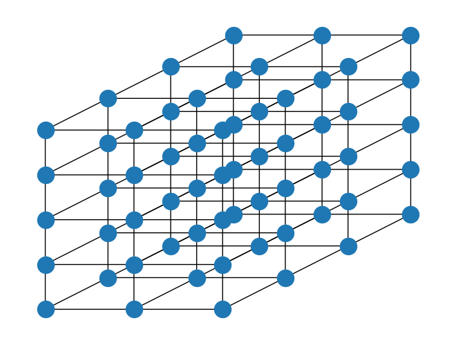
HyperCubicLattice#
HyperCubicLattice es una generalización de LineLattice y SquareLattice. Proporciona una retícula arbitraria d-dimensional. Aquí, hacemos una malla tridimensional de tamaño 3 por 4 por 5 como ejemplo. El tamaño se da como una tupla y las condiciones de frontera también se pueden especificar para cada dirección. En el ejemplo, las condiciones de frontera están abiertas.
[12]:
size = (3, 4, 5)
boundary_condition = (
    BoundaryCondition.OPEN,
    BoundaryCondition.OPEN,
    BoundaryCondition.OPEN,
)
cubic_lattice = HyperCubicLattice(size=size, boundary_condition=boundary_condition)
Dibujamos la retícula cúbica especificando las posiciones de los puntos de la malla.
[13]:
# function for setting the positions
def indextocoord_3d(index: int, size: tuple, angle) -> list:
    z = index // (size[0] * size[1])
    a = index % (size[0] * size[1])
    y = a // size[0]
    x = a % size[0]
    vec_x = np.array([1, 0])
    vec_y = np.array([np.cos(angle), np.sin(angle)])
    vec_z = np.array([0, 1])
    return_coord = x * vec_x + y * vec_y + z * vec_z
    return return_coord.tolist()


pos = dict([(index, indextocoord_3d(index, size, angle=pi / 4)) for index in range(np.prod(size))])

cubic_lattice.draw(style=LatticeDrawStyle(pos=pos))
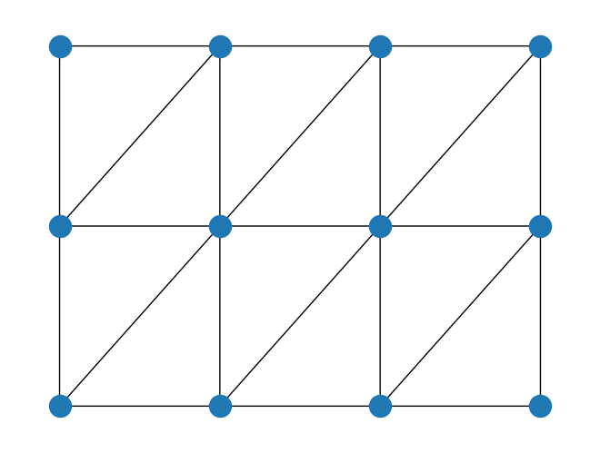
TriangularLattice#
TriangularLattice proporciona una retícula triangular, que puede verse como una malla bidimensional con bordes diagonales. El argumento boundary_condition puede tomar «open» o «periodic».
[14]:
rows = 4
cols = 3
boundary_condition = BoundaryCondition.OPEN

triangular_lattice = TriangularLattice(rows=rows, cols=cols, boundary_condition=boundary_condition)

triangular_lattice.draw()
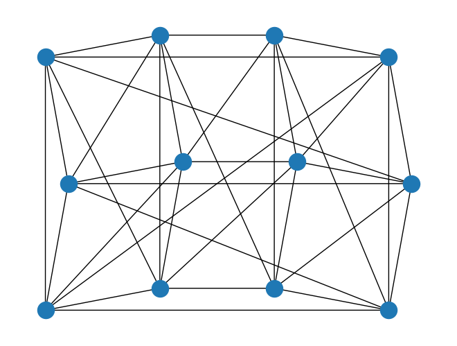
[15]:
rows = 4
cols = 3
boundary_condition = BoundaryCondition.PERIODIC

triangular_lattice = TriangularLattice(rows=rows, cols=cols, boundary_condition=boundary_condition)

triangular_lattice.draw()
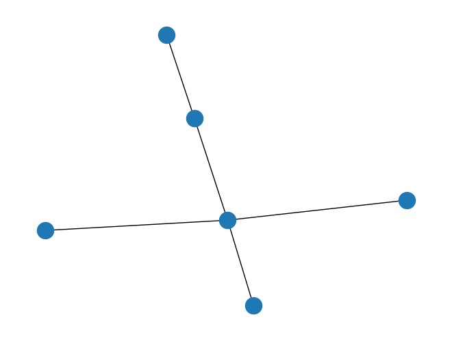
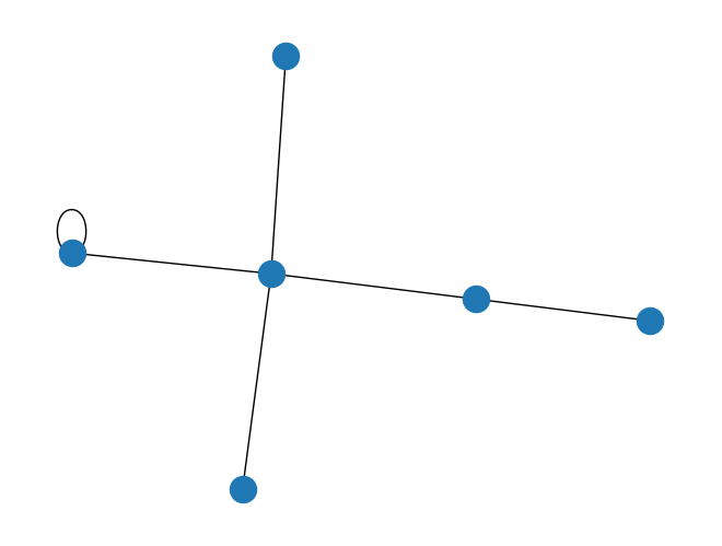
Retícula General#
Arriba, hemos visto retículas invariantes traslacionales. Aquí, consideramos una malla general. Podemos construir una retícula general que consta de nodos y bordes usando una instancia de PyGraph.
[16]:
graph = rx.PyGraph(multigraph=False)  # multigraph shoud be False
graph.add_nodes_from(range(6))
weighted_edge_list = [
    (0, 1, 1.0 + 1.0j),
    (0, 2, -1.0),
    (2, 3, 2.0),
    (4, 2, -1.0 + 2.0j),
    (4, 4, 3.0),
    (2, 5, -1.0),
]
graph.add_edges_from(weighted_edge_list)

# make a lattice
general_lattice = Lattice(graph)
set(general_lattice.graph.weighted_edge_list())
[16]:
{(0, 1, (1+1j)),
 (0, 2, -1.0),
 (2, 3, 2.0),
 (2, 5, -1.0),
 (4, 2, (-1+2j)),
 (4, 4, 3.0)}
Aquí está su visualización.
[17]:
general_lattice.draw()
Cuando queremos visualizar los auto-bucles en la retícula, configuramos self_loop con True.
[18]:
general_lattice.draw(self_loop=True)
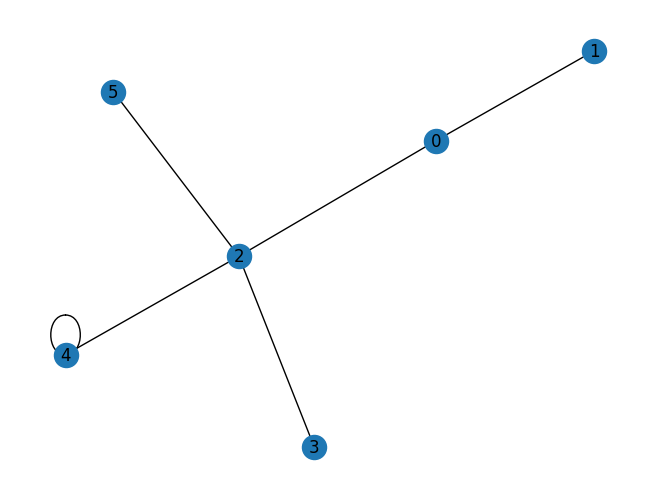
Las etiquetas de los sitios de la retícula se dibujan cuando with_labels es True.
[19]:
general_lattice.draw(self_loop=True, style=LatticeDrawStyle(with_labels=True))
El modelo Fermi-Hubbard#
El modelo de Fermi-Hubbard es el modelo más simple que describe los electrones que se mueven en una retícula e interactúan entre sí en el mismo sitio. El Hamiltoniano se da de la siguiente manera:
donde \(c_{i, \sigma}^\dagger\) y \(c_{i, \sigma}\) son operadores de creación y aniquilación de fermiones en el sitio \(i\) con espín \(\sigma\). El operador \(n_{i, \sigma}\) es el operador de número, que está definido por \(n_{i, \sigma} = c_{i, \sigma}^\dagger c_{i, \sigma}\). La matriz \(t_{i, j}\) es una matriz Hermitiana llamada matriz de interacción. El parámetro \(U\) representa la fuerza de la interacción.
Podemos generar el Hamiltoniano correspondiente de una retícula dada usando la clase FermiHubbardModel. Aquí, construimos el Hamiltoniano con interacción uniforme y parámetros de interacción en una malla bidimensional.
[20]:
square_lattice = SquareLattice(rows=5, cols=4, boundary_condition=BoundaryCondition.PERIODIC)

t = -1.0  # the interaction parameter
v = 0.0  # the onsite potential
u = 5.0  # the interaction parameter U

fhm = FermiHubbardModel(
    square_lattice.uniform_parameters(
        uniform_interaction=t,
        uniform_onsite_potential=v,
    ),
    onsite_interaction=u,
)
Para obtener el Hamiltoniano en términos de los operadores fermiónicos, usamos el método second_q_ops. El Hamiltoniano se devuelve como una instancia de FermionicOp.
Nota
El número de operadores fermiónicos requeridos es el doble del número de sitios de retícula debido a los grados de libertad del espín.
En la implementación, los índices pares corresponden a un espín arriba y los índices impares a un espín abajo.
[21]:
ham = fhm.second_q_op().simplify()
print(ham)
Fermionic Operator
number spin orbitals=40, number terms=180
  (-1+0j) * ( +_0 -_2 )
+ (1+0j) * ( -_0 +_2 )
+ (-1+0j) * ( +_0 -_10 )
+ (1+0j) * ( -_0 +_10 )
+ (-1+0j) * ( +_10 -_12 )
+ (1+0j) * ( -_10 +_12 )
+ (-1+0j) * ( +_10 -_20 )
+ (1+0j) * ( -_10 +_20 )
+ (-1+0j) * ( +_20 -_22 )
+ (1+0j) * ( -_20 +_22 )
+ (-1+0j) * ( +_20 -_30 )
+ (1+0j) * ( -_20 +_30 )
+ (-1+0j) * ( +_30 -_32 )
+ (1+0j) * ( -_30 +_32 )
+ (-1+0j) * ( +_2 -_4 )
+ (1+0j) * ( -_2 +_4 )
+ (-1+0j) * ( +_2 -_12 )
+ (1+0j) * ( -_2 +_12 )
+ (-1+0j) * ( +_12 -_14 )
+ (1+0j) * ( -_12 +_14 )
+ (-1+0j) * ( +_12 -_22 )
+ (1+0j) * ( -_12 +_22 )
+ (-1+0j) * ( +_22 -_24 )
+ (1+0j) * ( -_22 +_24 )
+ (-1+0j) * ( +_22 -_32 )
+ (1+0j) * ( -_22 +_32 )
+ (-1+0j) * ( +_32 -_34 )
+ (1+0j) * ( -_32 +_34 )
+ (-1+0j) * ( +_4 -_6 )
+ (1+0j) * ( -_4 +_6 )
+ (-1+0j) * ( +_4 -_14 )
+ (1+0j) * ( -_4 +_14 )
+ (-1+0j) * ( +_14 -_16 )
+ (1+0j) * ( -_14 +_16 )
+ (-1+0j) * ( +_14 -_24 )
+ (1+0j) * ( -_14 +_24 )
+ (-1+0j) * ( +_24 -_26 )
+ (1+0j) * ( -_24 +_26 )
+ (-1+0j) * ( +_24 -_34 )
+ (1+0j) * ( -_24 +_34 )
+ (-1+0j) * ( +_34 -_36 )
+ (1+0j) * ( -_34 +_36 )
+ (-1+0j) * ( +_6 -_8 )
+ (1+0j) * ( -_6 +_8 )
+ (-1+0j) * ( +_6 -_16 )
+ (1+0j) * ( -_6 +_16 )
+ (-1+0j) * ( +_16 -_18 )
+ (1+0j) * ( -_16 +_18 )
+ (-1+0j) * ( +_16 -_26 )
+ (1+0j) * ( -_16 +_26 )
+ (-1+0j) * ( +_26 -_28 )
+ (1+0j) * ( -_26 +_28 )
+ (-1+0j) * ( +_26 -_36 )
+ (1+0j) * ( -_26 +_36 )
+ (-1+0j) * ( +_36 -_38 )
+ (1+0j) * ( -_36 +_38 )
+ (-1+0j) * ( +_8 -_18 )
+ (1+0j) * ( -_8 +_18 )
+ (-1+0j) * ( +_18 -_28 )
+ (1+0j) * ( -_18 +_28 )
+ (-1+0j) * ( +_28 -_38 )
+ (1+0j) * ( -_28 +_38 )
+ (-1+0j) * ( +_0 -_8 )
+ (1+0j) * ( -_0 +_8 )
+ (-1+0j) * ( +_10 -_18 )
+ (1+0j) * ( -_10 +_18 )
+ (-1+0j) * ( +_20 -_28 )
+ (1+0j) * ( -_20 +_28 )
+ (-1+0j) * ( +_30 -_38 )
+ (1+0j) * ( -_30 +_38 )
+ (-1+0j) * ( +_0 -_30 )
+ (1+0j) * ( -_0 +_30 )
+ (-1+0j) * ( +_2 -_32 )
+ (1+0j) * ( -_2 +_32 )
+ (-1+0j) * ( +_4 -_34 )
+ (1+0j) * ( -_4 +_34 )
+ (-1+0j) * ( +_6 -_36 )
+ (1+0j) * ( -_6 +_36 )
+ (-1+0j) * ( +_8 -_38 )
+ (1+0j) * ( -_8 +_38 )
+ (-1+0j) * ( +_1 -_3 )
+ (1+0j) * ( -_1 +_3 )
+ (-1+0j) * ( +_1 -_11 )
+ (1+0j) * ( -_1 +_11 )
+ (-1+0j) * ( +_11 -_13 )
+ (1+0j) * ( -_11 +_13 )
+ (-1+0j) * ( +_11 -_21 )
+ (1+0j) * ( -_11 +_21 )
+ (-1+0j) * ( +_21 -_23 )
+ (1+0j) * ( -_21 +_23 )
+ (-1+0j) * ( +_21 -_31 )
+ (1+0j) * ( -_21 +_31 )
+ (-1+0j) * ( +_31 -_33 )
+ (1+0j) * ( -_31 +_33 )
+ (-1+0j) * ( +_3 -_5 )
+ (1+0j) * ( -_3 +_5 )
+ (-1+0j) * ( +_3 -_13 )
+ (1+0j) * ( -_3 +_13 )
+ (-1+0j) * ( +_13 -_15 )
+ (1+0j) * ( -_13 +_15 )
+ (-1+0j) * ( +_13 -_23 )
+ (1+0j) * ( -_13 +_23 )
+ (-1+0j) * ( +_23 -_25 )
+ (1+0j) * ( -_23 +_25 )
+ (-1+0j) * ( +_23 -_33 )
+ (1+0j) * ( -_23 +_33 )
+ (-1+0j) * ( +_33 -_35 )
+ (1+0j) * ( -_33 +_35 )
+ (-1+0j) * ( +_5 -_7 )
+ (1+0j) * ( -_5 +_7 )
+ (-1+0j) * ( +_5 -_15 )
+ (1+0j) * ( -_5 +_15 )
+ (-1+0j) * ( +_15 -_17 )
+ (1+0j) * ( -_15 +_17 )
+ (-1+0j) * ( +_15 -_25 )
+ (1+0j) * ( -_15 +_25 )
+ (-1+0j) * ( +_25 -_27 )
+ (1+0j) * ( -_25 +_27 )
+ (-1+0j) * ( +_25 -_35 )
+ (1+0j) * ( -_25 +_35 )
+ (-1+0j) * ( +_35 -_37 )
+ (1+0j) * ( -_35 +_37 )
+ (-1+0j) * ( +_7 -_9 )
+ (1+0j) * ( -_7 +_9 )
+ (-1+0j) * ( +_7 -_17 )
+ (1+0j) * ( -_7 +_17 )
+ (-1+0j) * ( +_17 -_19 )
+ (1+0j) * ( -_17 +_19 )
+ (-1+0j) * ( +_17 -_27 )
+ (1+0j) * ( -_17 +_27 )
+ (-1+0j) * ( +_27 -_29 )
+ (1+0j) * ( -_27 +_29 )
+ (-1+0j) * ( +_27 -_37 )
+ (1+0j) * ( -_27 +_37 )
+ (-1+0j) * ( +_37 -_39 )
+ (1+0j) * ( -_37 +_39 )
+ (-1+0j) * ( +_9 -_19 )
+ (1+0j) * ( -_9 +_19 )
+ (-1+0j) * ( +_19 -_29 )
+ (1+0j) * ( -_19 +_29 )
+ (-1+0j) * ( +_29 -_39 )
+ (1+0j) * ( -_29 +_39 )
+ (-1+0j) * ( +_1 -_9 )
+ (1+0j) * ( -_1 +_9 )
+ (-1+0j) * ( +_11 -_19 )
+ (1+0j) * ( -_11 +_19 )
+ (-1+0j) * ( +_21 -_29 )
+ (1+0j) * ( -_21 +_29 )
+ (-1+0j) * ( +_31 -_39 )
+ (1+0j) * ( -_31 +_39 )
+ (-1+0j) * ( +_1 -_31 )
+ (1+0j) * ( -_1 +_31 )
+ (-1+0j) * ( +_3 -_33 )
+ (1+0j) * ( -_3 +_33 )
+ (-1+0j) * ( +_5 -_35 )
+ (1+0j) * ( -_5 +_35 )
+ (-1+0j) * ( +_7 -_37 )
+ (1+0j) * ( -_7 +_37 )
+ (-1+0j) * ( +_9 -_39 )
+ (1+0j) * ( -_9 +_39 )
+ (5+0j) * ( +_0 -_0 +_1 -_1 )
+ (5+0j) * ( +_2 -_2 +_3 -_3 )
+ (5+0j) * ( +_4 -_4 +_5 -_5 )
+ (5+0j) * ( +_6 -_6 +_7 -_7 )
+ (5+0j) * ( +_8 -_8 +_9 -_9 )
+ (5+0j) * ( +_10 -_10 +_11 -_11 )
+ (5+0j) * ( +_12 -_12 +_13 -_13 )
+ (5+0j) * ( +_14 -_14 +_15 -_15 )
+ (5+0j) * ( +_16 -_16 +_17 -_17 )
+ (5+0j) * ( +_18 -_18 +_19 -_19 )
+ (5+0j) * ( +_20 -_20 +_21 -_21 )
+ (5+0j) * ( +_22 -_22 +_23 -_23 )
+ (5+0j) * ( +_24 -_24 +_25 -_25 )
+ (5+0j) * ( +_26 -_26 +_27 -_27 )
+ (5+0j) * ( +_28 -_28 +_29 -_29 )
+ (5+0j) * ( +_30 -_30 +_31 -_31 )
+ (5+0j) * ( +_32 -_32 +_33 -_33 )
+ (5+0j) * ( +_34 -_34 +_35 -_35 )
+ (5+0j) * ( +_36 -_36 +_37 -_37 )
+ (5+0j) * ( +_38 -_38 +_39 -_39 )
Lattice tiene pesos en sus bordes, por lo que podemos definir una matriz de interacción general utilizando una instancia de Lattice. Aquí, consideramos el modelo de Fermi-Hubbard en una retícula general en la que se dan parámetros de interacción no uniformes. En este caso, los pesos de la retícula se consideran la matriz de interacción. Después de generar el Hamiltoniano (second_q_ops) podemos usar un mapeador de qubit para generar los operadores de qubit y/o usar cualquiera de los algoritmos disponibles para resolver el problema de retícula correspondiente.
[22]:
graph = rx.PyGraph(multigraph=False)  # multiigraph shoud be False
graph.add_nodes_from(range(6))
weighted_edge_list = [
    (0, 1, 1.0 + 1.0j),
    (0, 2, -1.0),
    (2, 3, 2.0),
    (4, 2, -1.0 + 2.0j),
    (4, 4, 3.0),
    (2, 5, -1.0),
]
graph.add_edges_from(weighted_edge_list)

general_lattice = Lattice(graph)  # the lattice whose weights are seen as the interaction matrix.
u = 5.0  # the interaction parameter U

fhm = FermiHubbardModel(lattice=general_lattice, onsite_interaction=u)

ham = fhm.second_q_op().simplify()
print(ham)
Fermionic Operator
number spin orbitals=12, number terms=28
  (1+1j) * ( +_0 -_2 )
+ (-1+1j) * ( -_0 +_2 )
+ (-1+0j) * ( +_0 -_4 )
+ (1+0j) * ( -_0 +_4 )
+ (2+0j) * ( +_4 -_6 )
+ (-2+0j) * ( -_4 +_6 )
+ (-1-2j) * ( +_4 -_8 )
+ (1-2j) * ( -_4 +_8 )
+ (3+0j) * ( +_8 -_8 )
+ (-1+0j) * ( +_4 -_10 )
+ (1+0j) * ( -_4 +_10 )
+ (1+1j) * ( +_1 -_3 )
+ (-1+1j) * ( -_1 +_3 )
+ (-1+0j) * ( +_1 -_5 )
+ (1+0j) * ( -_1 +_5 )
+ (2+0j) * ( +_5 -_7 )
+ (-2+0j) * ( -_5 +_7 )
+ (-1-2j) * ( +_5 -_9 )
+ (1-2j) * ( -_5 +_9 )
+ (3+0j) * ( +_9 -_9 )
+ (-1+0j) * ( +_5 -_11 )
+ (1+0j) * ( -_5 +_11 )
+ (5+0j) * ( +_0 -_0 +_1 -_1 )
+ (5+0j) * ( +_2 -_2 +_3 -_3 )
+ (5+0j) * ( +_4 -_4 +_5 -_5 )
+ (5+0j) * ( +_6 -_6 +_7 -_7 )
+ (5+0j) * ( +_8 -_8 +_9 -_9 )
+ (5+0j) * ( +_10 -_10 +_11 -_11 )
LatticeModelProblem#
Qiskit Nature también tiene una clase LatticeModelProblem que permite el uso del GroundStateEigensolver para calcular la energía del estado fundamental de una retícula determinada. Puedes usar esta clase de la siguiente manera:
[23]:
from qiskit_nature.second_q.problems import LatticeModelProblem

num_nodes = 4
boundary_condition = BoundaryCondition.OPEN
line_lattice = LineLattice(num_nodes=num_nodes, boundary_condition=boundary_condition)

fhm = FermiHubbardModel(
    line_lattice.uniform_parameters(
        uniform_interaction=t,
        uniform_onsite_potential=v,
    ),
    onsite_interaction=u,
)

lmp = LatticeModelProblem(fhm)
[24]:
from qiskit_algorithms import NumPyMinimumEigensolver
from qiskit_nature.second_q.algorithms import GroundStateEigensolver
from qiskit_nature.second_q.mappers import JordanWignerMapper

numpy_solver = NumPyMinimumEigensolver()

qubit_mapper = JordanWignerMapper()

calc = GroundStateEigensolver(qubit_mapper, numpy_solver)
res = calc.solve(lmp)

print(res)
=== GROUND STATE ===

* Lattice ground state energy : -2.566350190841
[25]:
import qiskit.tools.jupyter

%qiskit_version_table
%qiskit_copyright
Version Information
| Qiskit Software | Version |
|---|---|
qiskit-terra | 0.24.0.dev0+2b3686f |
qiskit-aer | 0.11.2 |
qiskit-ibmq-provider | 0.19.2 |
qiskit-nature | 0.6.0 |
| System information | |
| Python version | 3.9.16 |
| Python compiler | GCC 12.2.1 20221121 (Red Hat 12.2.1-4) |
| Python build | main, Dec 7 2022 00:00:00 |
| OS | Linux |
| CPUs | 8 |
| Memory (Gb) | 62.50002670288086 |
| Thu Apr 06 09:13:58 2023 CEST | |
This code is a part of Qiskit
© Copyright IBM 2017, 2023.
This code is licensed under the Apache License, Version 2.0. You may
obtain a copy of this license in the LICENSE.txt file in the root directory
of this source tree or at http://www.apache.org/licenses/LICENSE-2.0.
Any modifications or derivative works of this code must retain this
copyright notice, and modified files need to carry a notice indicating
that they have been altered from the originals.