Note
இந்தப் பக்கம் docs/tutorials/௦௯_saving_and_loading_models.app சட்டத்தால் உருவாக்கப்பட்டது.
சேமிப்பு, கிஸ்கிட் இயந்திர கற்றல் மாதிரிகளை ஏற்றுதல் மற்றும் தொடர்ச்சியான பயிற்சி#
இந்த டுடோரியலில் Qiskit இயந்திர கற்றல் மாதிரிகளை எவ்வாறு சேமிப்பது மற்றும் ஏற்றுவது என்பதைக் காண்பிப்போம். ஒரு மாதிரியைச் சேமிக்கும் திறன் மிகவும் முக்கியமானது, குறிப்பாக உண்மையான வன்பொருளில் ஒரு மாதிரியைப் பயிற்றுவிப்பதில் கணிசமான அளவு நேரத்தை முதலீடு செய்யும் போது. மேலும், முன்பு சேமித்த மாதிரியின் பயிற்சியை எவ்வாறு மீண்டும் தொடங்குவது என்பதை நாங்கள் காண்பிப்போம்.
இந்த டுடோரியலில், எப்படி செய்வது என்று பார்ப்போம்:
எளிய தரவுத்தொகுப்பை உருவாக்கி, அதை பயிற்சி/சோதனை தரவுத்தொகுப்புகளாகப் பிரித்து அவற்றைத் திட்டமிடுங்கள்
ஒரு மாதிரியைப் பயிற்றுவித்துச் சேமிக்கவும்
சேமித்த மாதிரியை ஏற்றிப் பயிற்சியை மீண்டும் தொடங்கவும்
மாதிரிகளின் செயல்திறனை மதிப்பிடுங்கள்
பைடார்ச் கலப்பின மாதிரிகள்
First off, we start from the required imports. We’ll heavily use SciKit-Learn on the data preparation step. In the next cell we also fix a random seed for reproducibility purposes.
[1]:
import matplotlib.pyplot as plt
import numpy as np
from qiskit.circuit.library import RealAmplitudes
from qiskit.primitives import Sampler
from qiskit_algorithms.optimizers import COBYLA
from qiskit_algorithms.utils import algorithm_globals
from sklearn.model_selection import train_test_split
from sklearn.preprocessing import OneHotEncoder, MinMaxScaler

from qiskit_machine_learning.algorithms.classifiers import VQC

from IPython.display import clear_output

algorithm_globals.random_seed = 42
We will be using two quantum simulators, in particular, two instances of the Sampler primitive. We’ll start training on the first one, then will resume training on the second one. The approach shown in this tutorial can be used to train a model on a real hardware available on the cloud and then re-use the model for inference on a local simulator.
[2]:
sampler1 = Sampler()

sampler2 = Sampler()
1. தரவுத்தொகுப்பைத் தயாரிக்கவும்#
அடுத்த படி தரவுத்தொகுப்பைத் தயாரிப்பது. மற்ற டுடோரியல்களைப் போலவே இங்கேயும் சில தரவுகளை உருவாக்குகிறோம். வித்தியாசம் என்னவென்றால், உருவாக்கப்பட்ட தரவுகளுக்கு சில மாற்றங்களைப் பயன்படுத்துகிறோம். நாங்கள் 40 மாதிரிகளை உருவாக்குகிறோம், ஒவ்வொரு மாதிரியிலும் 2 அம்சங்கள் உள்ளன, எனவே எங்கள் அம்சங்கள் (40, 2) வடிவத்தின் வரிசையாகும். நெடுவரிசைகள் மூலம் அம்சங்களைச் சுருக்கி லேபிள்கள் பெறப்படுகின்றன, மேலும் கூட்டுத்தொகை 1``க்கு அதிகமாக இருந்தால், இந்த மாதிரி ``1 மற்றும் 0 என லேபிளிடப்படும்.
[3]:
num_samples = 40
num_features = 2
features = 2 * algorithm_globals.random.random([num_samples, num_features]) - 1
labels = 1 * (np.sum(features, axis=1) >= 0)  # in { 0,  1}
பிறகு, SciKit-Learn இலிருந்து MinMaxScaler ஐப் பயன்படுத்துவதன் மூலம் எங்கள் அம்சங்களை [0, 1] வரம்பிற்குள் அளவிடுகிறோம். இந்த மாற்றம் பயன்படுத்தப்படும்போது மாதிரிப் பயிற்சி ஒருங்கிணைப்பு சிறப்பாக இருக்கும்.
[4]:
features = MinMaxScaler().fit_transform(features)
features.shape
[4]:
(40, 2)
Let’s take a look at the features of the first 5 samples of our dataset after the transformation.
[5]:
features[0:5, :]
[5]:
array([[0.79067335, 0.44566143],
       [0.88072937, 0.7126244 ],
       [0.06741233, 1.        ],
       [0.7770372 , 0.80422817],
       [0.10351936, 0.45754615]])
நாங்கள் பயிற்சியளிக்கும் மாதிரியாக VQC` அல்லது மாறுபாடு குவாண்டம் வகைப்படுத்தியைத் தேர்வு செய்கிறோம். இந்த மாதிரி, இயல்பாக, ஒரு சூடான குறியிடப்பட்ட லேபிள்களை எடுக்கும், எனவே ``{0, 1} தொகுப்பில் உள்ள லேபிள்களை ஒரு சூடான பிரதிநிதித்துவமாக மாற்ற வேண்டும். இந்த மாற்றத்திற்கும் நாங்கள் SciKit-Learn ஐப் பயன்படுத்துகிறோம். உள்ளீட்டு அணிவரிசை முதலில் (num_samples, 1) என மறுவடிவமைக்கப்பட வேண்டும் என்பதை நினைவில் கொள்ளவும். OneHotEncoder குறியாக்கி 1D வரிசைகளுடன் வேலை செய்யாது மற்றும் எங்கள் லேபிள்கள் 1D வரிசையாகும். இந்த வழக்கில், ஒரு வரிசைக்கு ஒரே ஒரு அம்சம் (எங்கள் வழக்கு!) அல்லது ஒரு மாதிரி உள்ளது என்பதை பயனர் தீர்மானிக்க வேண்டும். மேலும், முன்னிருப்பாக, குறியாக்கி அரிதான வரிசைகளை வழங்குகிறது, ஆனால் தரவுத்தொகுப்பு திட்டமிடலுக்கு அடர்த்தியான வரிசைகளை வைத்திருப்பது எளிதாக இருக்கும், எனவே நாம் sparse என்பதை False` என அமைக்கிறோம்.
[6]:
labels = OneHotEncoder(sparse_output=False).fit_transform(labels.reshape(-1, 1))
labels.shape
[6]:
(40, 2)
Let’s take a look at the labels of the first 5 labels of the dataset. The labels should be one-hot encoded.
[7]:
labels[0:5, :]
[7]:
array([[0., 1.],
       [0., 1.],
       [0., 1.],
       [0., 1.],
       [1., 0.]])
இப்போது எங்கள் தரவுத்தொகுப்பை இரண்டு பகுதிகளாகப் பிரிக்கிறோம்: பயிற்சி தரவுத்தொகுப்பு மற்றும் சோதனை ஒன்று. கட்டைவிரல் விதியாக, முழு தரவுத்தொகுப்பில் 80% பயிற்சிப் பகுதியிலும் 20% சோதனையிலும் செல்ல வேண்டும். எங்கள் பயிற்சி தரவுத்தொகுப்பில் 30 மாதிரிகள் உள்ளன. சோதனை தரவுத்தொகுப்பு ஒரு முறை மட்டுமே பயன்படுத்தப்பட வேண்டும், மாடல் பார்க்காத தரவில் எவ்வளவு சிறப்பாக செயல்படுகிறது என்பதை சரிபார்க்க ஒரு மாதிரி பயிற்சி அளிக்கப்படும். நாங்கள் SciKit-Learn இலிருந்து Train_test_split ஐப் பயன்படுத்துகிறோம்.
[8]:
train_features, test_features, train_labels, test_labels = train_test_split(
    features, labels, train_size=30, random_state=algorithm_globals.random_seed
)
train_features.shape
[8]:
(30, 2)
Now it is time to see how our dataset looks like. Let’s plot it.
[9]:
def plot_dataset():
    plt.scatter(
        train_features[np.where(train_labels[:, 0] == 0), 0],
        train_features[np.where(train_labels[:, 0] == 0), 1],
        marker="o",
        color="b",
        label="Label 0 train",
    )
    plt.scatter(
        train_features[np.where(train_labels[:, 0] == 1), 0],
        train_features[np.where(train_labels[:, 0] == 1), 1],
        marker="o",
        color="g",
        label="Label 1 train",
    )

    plt.scatter(
        test_features[np.where(test_labels[:, 0] == 0), 0],
        test_features[np.where(test_labels[:, 0] == 0), 1],
        marker="o",
        facecolors="w",
        edgecolors="b",
        label="Label 0 test",
    )
    plt.scatter(
        test_features[np.where(test_labels[:, 0] == 1), 0],
        test_features[np.where(test_labels[:, 0] == 1), 1],
        marker="o",
        facecolors="w",
        edgecolors="g",
        label="Label 1 test",
    )

    plt.legend(bbox_to_anchor=(1.05, 1), loc="upper left", borderaxespad=0.0)
    plt.plot([1, 0], [0, 1], "--", color="black")


plot_dataset()
plt.show()
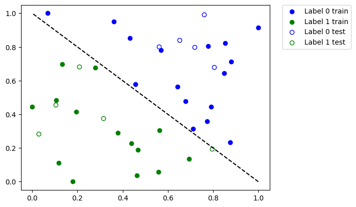
மேலே உள்ள சதியில் நாம் பார்க்கிறோம்:
திட நீல புள்ளிகள் என்பது
0எனப் பெயரிடப்பட்ட பயிற்சி தரவுத்தொகுப்பிலிருந்து மாதிரிகள்வெற்று நீல புள்ளிகள் என்பது
0என லேபிளிடப்பட்ட சோதனை தரவுத்தொகுப்பிலிருந்து மாதிரிகள்திட பச்சை புள்ளிகள் என்பது
1எனப் பெயரிடப்பட்ட பயிற்சி தரவுத்தொகுப்பிலிருந்து மாதிரிகள்வெற்று பச்சை புள்ளிகள் என்பது
1என லேபிளிடப்பட்ட சோதனை தரவுத்தொகுப்பிலிருந்து மாதிரிகள்
We’ll train our model using solid dots and verify it using empty dots.
2. ஒரு மாதிரியைப் பயிற்றுவித்து அதைச் சேமிக்கவும்#
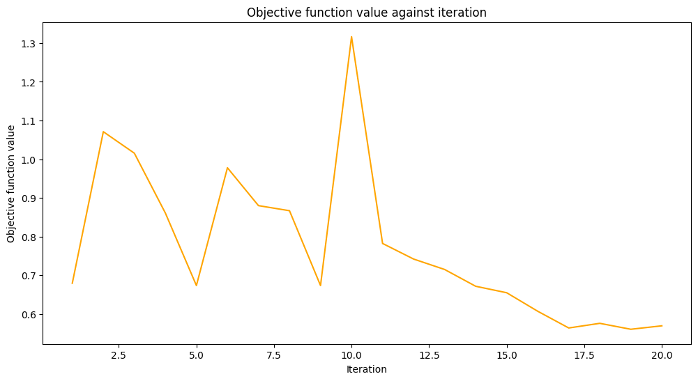
We’ll train our model in two steps. On the first step we train our model in 20 iterations.
[10]:
maxiter = 20
புறநிலை செயல்பாட்டின் மதிப்புகளைச் சேமிப்பதற்காகத் திரும்ப அழைப்பதற்கு வெற்று வரிசையை உருவாக்கவும்.
[11]:
objective_values = []
நியூரல் நெட்வொர்க் கிளாசிஃபையர் & ரீக்ரஸர் டுடோரியலிலிருந்து மீண்டும் கால்பேக் செயல்பாட்டைப் பயன்படுத்தி, ஒவ்வொரு அடியிலும் புறநிலை மதிப்புகளைத் திட்டமிடுவதற்கு சில சிறிய மாற்றங்களுடன் மறு செய்கை மற்றும் புறநிலை செயல்பாடு மதிப்பைத் திட்டமிடுவோம்.
[12]:
# callback function that draws a live plot when the .fit() method is called
def callback_graph(_, objective_value):
    clear_output(wait=True)
    objective_values.append(objective_value)

    plt.title("Objective function value against iteration")
    plt.xlabel("Iteration")
    plt.ylabel("Objective function value")

    stage1_len = np.min((len(objective_values), maxiter))
    stage1_x = np.linspace(1, stage1_len, stage1_len)
    stage1_y = objective_values[:stage1_len]

    stage2_len = np.max((0, len(objective_values) - maxiter))
    stage2_x = np.linspace(maxiter, maxiter + stage2_len - 1, stage2_len)
    stage2_y = objective_values[maxiter : maxiter + stage2_len]

    plt.plot(stage1_x, stage1_y, color="orange")
    plt.plot(stage2_x, stage2_y, color="purple")
    plt.show()


plt.rcParams["figure.figsize"] = (12, 6)
மேலே குறிப்பிட்டுள்ளபடி, VQC மாதிரியைப் பயிற்றுவித்து, maxiter அளவுருவின் தேர்ந்தெடுக்கப்பட்ட மதிப்பைக் கொண்டு COBYLA ஐ ஆப்டிமைசராக அமைக்கிறோம். மாதிரியின் செயல்திறன் எவ்வளவு நன்றாகப் பயிற்றுவிக்கப்பட்டது என்பதைப் பார்க்க, அதன் செயல்திறனை மதிப்பீடு செய்கிறோம். இந்த மாதிரியை ஒரு கோப்பிற்காக சேமிக்கிறோம். இரண்டாவது கட்டத்தில், இந்த மாதிரியை ஏற்றுகிறோம், அதனுடன் தொடர்ந்து வேலை செய்வோம்.
இங்கே, மேம்படுத்தலைத் தொடங்குவதற்கான ஆரம்பப் புள்ளியைச் சரிசெய்ய, ஒரு ansatz ஐ கைமுறையாக உருவாக்குகிறோம்.
[13]:
original_optimizer = COBYLA(maxiter=maxiter)

ansatz = RealAmplitudes(num_features)
initial_point = np.asarray([0.5] * ansatz.num_parameters)
நாங்கள் ஒரு மாதிரியை உருவாக்கி, முன்பு உருவாக்கிய முதல் மாதிரிக்கு ஒரு மாதிரியை அமைக்கிறோம்.
[14]:
original_classifier = VQC(
    ansatz=ansatz, optimizer=original_optimizer, callback=callback_graph, sampler=sampler1
)
இப்போது மாதிரியைப் பயிற்றுவிப்பதற்கான நேரம் இது.
[15]:
original_classifier.fit(train_features, train_labels)
[15]:
<qiskit_machine_learning.algorithms.classifiers.vqc.VQC at 0x7fb74126db20>
Let’s see how well our model performs after the first step of training.
[16]:
print("Train score", original_classifier.score(train_features, train_labels))
print("Test score ", original_classifier.score(test_features, test_labels))
Train score 0.8333333333333334
Test score  0.8
அடுத்து, மாதிரியைச் சேமிக்கிறோம். நீங்கள் விரும்பும் எந்தக் கோப்பு பெயரையும் தேர்வு செய்யலாம். கோப்பு பெயரில் குறிப்பிடப்படாவிட்டால், save முறை நீட்டிப்பைச் சேர்க்காது என்பதை நினைவில் கொள்ளவும்.
[17]:
original_classifier.save("vqc_classifier.model")
3. ஒரு மாதிரியை ஏற்றிப் பயிற்சியைத் தொடரவும்#
ஒரு மாதிரியை ஏற்றுவதற்கு, ஒரு பயனர், தொடர்புடைய மாதிரி வகுப்பின் வகுப்பு முறையை load என்று அழைக்க வேண்டும். எங்கள் விஷயத்தில் அது VQC. எங்கள் மாதிரியைச் சேமித்த முந்தைய பிரிவில் நாங்கள் பயன்படுத்திய அதே கோப்புப் பெயரை நாங்கள் அனுப்புகிறோம்.
[18]:
loaded_classifier = VQC.load("vqc_classifier.model")
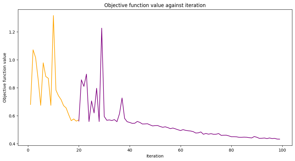
அடுத்து, மாடலை மேலும் மற்றும் மற்றொரு சிமுலேட்டரில் பயிற்சியளிக்கக்கூடிய வகையில் மாற்ற விரும்புகிறோம். அவ்வாறு செய்ய, warm_start சொத்தை அமைக்கிறோம். இது True என அமைக்கப்பட்டு fit() என அழைக்கப்படும் போது, மாடல் புதிய பொருத்தத்தைத் தொடங்க முந்தைய பொருத்தத்தின் எடையைப் பயன்படுத்துகிறது. டுடோரியலின் தொடக்கத்தில் நாங்கள் உருவாக்கிய sampler ப்ரிமிட்டிவ் இன் இரண்டாவது நிகழ்வாக அடிப்படை நெட்வொர்க்கின் Sampler பண்புகளையும் அமைத்துள்ளோம். இறுதியாக, maxiter 80 என அமைக்கப்பட்ட புதிய ஆப்டிமைசரை உருவாக்கி அமைக்கிறோம், எனவே மொத்த மறு செய்கைகளின் எண்ணிக்கை 100 ஆகும்.
[19]:
loaded_classifier.warm_start = True
loaded_classifier.neural_network.sampler = sampler2
loaded_classifier.optimizer = COBYLA(maxiter=80)
இப்போது நாங்கள் முந்தைய பிரிவில் முடித்த மாநிலத்திலிருந்து எங்கள் மாதிரியைத் தொடர்ந்து பயிற்சி செய்கிறோம்.
[20]:
loaded_classifier.fit(train_features, train_labels)
[20]:
<qiskit_machine_learning.algorithms.classifiers.vqc.VQC at 0x7fb7411cb760>
[21]:
print("Train score", loaded_classifier.score(train_features, train_labels))
print("Test score", loaded_classifier.score(test_features, test_labels))
Train score 0.9
Test score 0.8
Let’s see which data points were misclassified. First, we call predict to infer predicted values from the training and test features.
[22]:
train_predicts = loaded_classifier.predict(train_features)
test_predicts = loaded_classifier.predict(test_features)
முழு தரவுத்தொகுப்பையும் வரைந்து, தவறாக வகைப்படுத்தப்பட்ட புள்ளிகளை முன்னிலைப்படுத்தவும்.
[23]:
# return plot to default figsize
plt.rcParams["figure.figsize"] = (6, 4)

plot_dataset()

# plot misclassified data points
plt.scatter(
    train_features[np.all(train_labels != train_predicts, axis=1), 0],
    train_features[np.all(train_labels != train_predicts, axis=1), 1],
    s=200,
    facecolors="none",
    edgecolors="r",
    linewidths=2,
)
plt.scatter(
    test_features[np.all(test_labels != test_predicts, axis=1), 0],
    test_features[np.all(test_labels != test_predicts, axis=1), 1],
    s=200,
    facecolors="none",
    edgecolors="r",
    linewidths=2,
)
[23]:
<matplotlib.collections.PathCollection at 0x7fb6e04c2eb0>
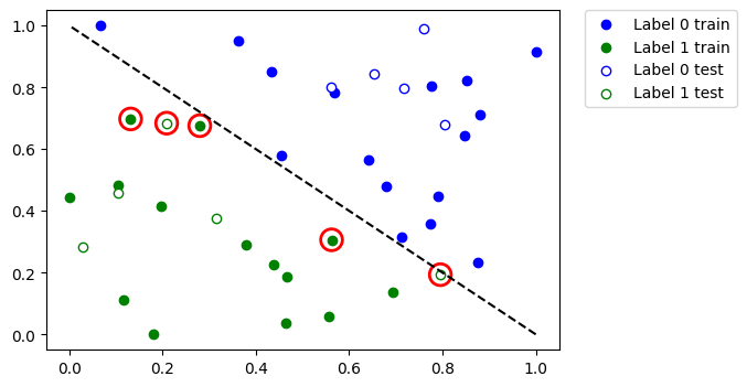
எனவே, உங்களிடம் பெரிய தரவுத்தொகுப்பு அல்லது பெரிய மாதிரி இருந்தால், இந்த டுடோரியலில் காட்டப்பட்டுள்ளபடி அதைப் பல படிகளில் பயிற்சி செய்யலாம்.
4. PyTorch கலப்பின மாதிரிகள்#
To save and load hybrid models, when using the TorchConnector, follow the PyTorch recommendations of saving and loading the models. For more details please refer to the PyTorch Connector tutorial where a short snippet shows how to do it.
யோசனையைப் பெற இந்தப் போலி போன்ற குறியீட்டைப் பாருங்கள்:
# create a QNN and a hybrid model
qnn = create_qnn()
model = Net(qnn)
# ... train the model ...

# save the model
torch.save(model.state_dict(), "model.pt")

# create a new model
new_qnn = create_qnn()
loaded_model = Net(new_qnn)
loaded_model.load_state_dict(torch.load("model.pt"))
[24]:
import qiskit.tools.jupyter

%qiskit_version_table
%qiskit_copyright
Version Information
| Qiskit Software | Version |
|---|---|
qiskit-terra | 0.25.0 |
qiskit-aer | 0.13.0 |
qiskit-machine-learning | 0.7.0 |
| System information | |
| Python version | 3.8.13 |
| Python compiler | Clang 12.0.0 |
| Python build | default, Oct 19 2022 17:54:22 |
| OS | Darwin |
| CPUs | 10 |
| Memory (Gb) | 64.0 |
| Mon Jun 12 11:51:03 2023 IST | |
This code is a part of Qiskit
© Copyright IBM 2017, 2023.
This code is licensed under the Apache License, Version 2.0. You may
obtain a copy of this license in the LICENSE.txt file in the root directory
of this source tree or at http://www.apache.org/licenses/LICENSE-2.0.
Any modifications or derivative works of this code must retain this
copyright notice, and modified files need to carry a notice indicating
that they have been altered from the originals.