Note
இந்தப் பக்கம் docs/tutorials/08_quantum_kernel_trainer.ipynb இல்லிருந்து உருவாக்கப்பட்டது.
இயந்திர கற்றல் பயன்பாடுகளுக்கான குவாண்டம் கர்னல் பயிற்சி#
In this tutorial, we will train a quantum kernel on a labeled dataset for a machine learning application. To illustrate the basic steps, we will use Quantum Kernel Alignment (QKA) for a binary classification task. QKA is a technique that iteratively adapts a parametrized quantum kernel to a dataset while converging to the maximum SVM margin. More information about QKA can be found in the preprint, "Covariant quantum kernels for data with group structure."
குவாண்டம் கர்னலைப் பயிற்றுவிப்பதற்கான நுழைவுப் புள்ளி QuantumKernelTrainer வகுப்பாகும். அடிப்படை படிகள்:
தரவுத்தொகுப்பைத் தயாரிக்கவும்
குவாண்டம் அம்ச வரைபடத்தை வரையறுக்கவும்
Set up an instance of
TrainableKernelandQuantumKernelTrainerobjectsதரவுத்தொகுப்பில் கர்னல் அளவுருக்களைப் பயிற்றுவிக்க
QuantumKernelTrainer.fitமுறையைப் பயன்படுத்தவும்பயிற்சி பெற்ற குவாண்டம் கர்னலை இயந்திர கற்றல் மாதிரிக்கு அனுப்பவும்
உள்ளூர், வெளி மற்றும் கிஸ்கிட் தொகுப்புகளை இறக்குமதி செய்து, எங்கள் ஆப்டிமைசருக்கான கால்பேக் வகுப்பை வரையறுக்கவும்#
[1]:
# External imports
from pylab import cm
from sklearn import metrics
import numpy as np
import matplotlib
import matplotlib.pyplot as plt

# Qiskit imports
from qiskit import QuantumCircuit
from qiskit.circuit import ParameterVector
from qiskit.visualization import circuit_drawer
from qiskit.circuit.library import ZZFeatureMap
from qiskit_algorithms.optimizers import SPSA
from qiskit_machine_learning.kernels import TrainableFidelityQuantumKernel
from qiskit_machine_learning.kernels.algorithms import QuantumKernelTrainer
from qiskit_machine_learning.algorithms import QSVC
from qiskit_machine_learning.datasets import ad_hoc_data


class QKTCallback:
    """Callback wrapper class."""

    def __init__(self) -> None:
        self._data = [[] for i in range(5)]

    def callback(self, x0, x1=None, x2=None, x3=None, x4=None):
        """
        Args:
            x0: number of function evaluations
            x1: the parameters
            x2: the function value
            x3: the stepsize
            x4: whether the step was accepted
        """
        self._data[0].append(x0)
        self._data[1].append(x1)
        self._data[2].append(x2)
        self._data[3].append(x3)
        self._data[4].append(x4)

    def get_callback_data(self):
        return self._data

    def clear_callback_data(self):
        self._data = [[] for i in range(5)]
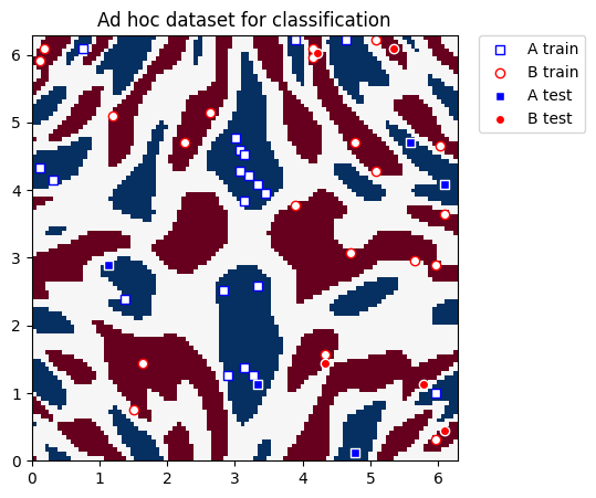
தரவுத்தொகுப்பைத் தயாரிக்கவும்#
In this guide, we will use Qiskit Machine Learning’s ad_hoc.py dataset to demonstrate the kernel training process. See the documentation here.
[2]:
adhoc_dimension = 2
X_train, y_train, X_test, y_test, adhoc_total = ad_hoc_data(
    training_size=20,
    test_size=5,
    n=adhoc_dimension,
    gap=0.3,
    plot_data=False,
    one_hot=False,
    include_sample_total=True,
)

plt.figure(figsize=(5, 5))
plt.ylim(0, 2 * np.pi)
plt.xlim(0, 2 * np.pi)
plt.imshow(
    np.asmatrix(adhoc_total).T,
    interpolation="nearest",
    origin="lower",
    cmap="RdBu",
    extent=[0, 2 * np.pi, 0, 2 * np.pi],
)

plt.scatter(
    X_train[np.where(y_train[:] == 0), 0],
    X_train[np.where(y_train[:] == 0), 1],
    marker="s",
    facecolors="w",
    edgecolors="b",
    label="A train",
)
plt.scatter(
    X_train[np.where(y_train[:] == 1), 0],
    X_train[np.where(y_train[:] == 1), 1],
    marker="o",
    facecolors="w",
    edgecolors="r",
    label="B train",
)
plt.scatter(
    X_test[np.where(y_test[:] == 0), 0],
    X_test[np.where(y_test[:] == 0), 1],
    marker="s",
    facecolors="b",
    edgecolors="w",
    label="A test",
)
plt.scatter(
    X_test[np.where(y_test[:] == 1), 0],
    X_test[np.where(y_test[:] == 1), 1],
    marker="o",
    facecolors="r",
    edgecolors="w",
    label="B test",
)

plt.legend(bbox_to_anchor=(1.05, 1), loc="upper left", borderaxespad=0.0)
plt.title("Ad hoc dataset for classification")

plt.show()
குவாண்டம் அம்ச வரைபடத்தை வரையறுக்கவும்#
அடுத்து, நாங்கள் குவாண்டம் அம்ச வரைபடத்தை அமைக்கிறோம், இது கிளாசிக்கல் தரவைக் குவாண்டம் நிலை இடத்தில் குறியாக்குகிறது. இங்கே, பயிற்சியளிக்கக்கூடிய சுழற்சி அடுக்கை அமைக்க QuantumCircuit மற்றும் உள்ளீட்டுத் தரவைக் குறிக்க Qiskit இலிருந்து ZZFeatureMap ஐப் பயன்படுத்துகிறோம்.
[3]:
# Create a rotational layer to train. We will rotate each qubit the same amount.
training_params = ParameterVector("θ", 1)
fm0 = QuantumCircuit(2)
fm0.ry(training_params[0], 0)
fm0.ry(training_params[0], 1)

# Use ZZFeatureMap to represent input data
fm1 = ZZFeatureMap(2)

# Create the feature map, composed of our two circuits
fm = fm0.compose(fm1)

print(circuit_drawer(fm))
print(f"Trainable parameters: {training_params}")
     ┌──────────┐┌──────────────────────────┐
q_0: ┤ Ry(θ[0]) ├┤0                         ├
     ├──────────┤│  ZZFeatureMap(x[0],x[1]) │
q_1: ┤ Ry(θ[0]) ├┤1                         ├
     └──────────┘└──────────────────────────┘
Trainable parameters: θ, ['θ[0]']
குவாண்டம் கர்னல் மற்றும் குவாண்டம் கர்னல் பயிற்சியாளரை அமைக்கவும்#
To train the quantum kernel, we will use an instance of TrainableFidelityQuantumKernel (holds the feature map and its parameters) and QuantumKernelTrainer (manages the training process).
QuantumKernelTrainer க்கு உள்ளீடாக, SVCLoss` என்ற கர்னல் இழப்புச் செயல்பாட்டைத் தேர்ந்தெடுப்பதன் மூலம் குவாண்டம் கர்னல் சீரமைப்பு நுட்பத்தைப் பயன்படுத்தி பயிற்சி அளிப்போம். இது Qiskit-ஆதரவு இழப்பாக இருப்பதால், "svc_loss" என்ற சரத்தைப் பயன்படுத்தலாம்; இருப்பினும், இழப்பை ஒரு சரமாக அனுப்பும்போது இயல்புநிலை அமைப்புகள் பயன்படுத்தப்படும் என்பதை நினைவில் கொள்ளவும். தனிப்பயன் அமைப்புகளுக்கு, விரும்பிய விருப்பங்களுடன் வெளிப்படையாகத் தெரிவிக்கவும், மேலும் KernelLoss பொருளை QuantumKernelTrainer க்கு அனுப்பவும்.
SPSA ஐ ஆப்டிமைசராகத் தேர்ந்தெடுத்து, பயிற்சியளிக்கக்கூடிய அளவுருவை initial_point வாதத்துடன் துவக்குவோம். குறிப்பு: initial_point வாதமாக அனுப்பப்பட்ட பட்டியலின் நீளம், அம்ச வரைபடத்தில் பயிற்சியளிக்கக்கூடிய அளவுருக்களின் எண்ணிக்கைக்குச் சமமாக இருக்க வேண்டும்.
[4]:
# Instantiate quantum kernel
quant_kernel = TrainableFidelityQuantumKernel(feature_map=fm, training_parameters=training_params)

# Set up the optimizer
cb_qkt = QKTCallback()
spsa_opt = SPSA(maxiter=10, callback=cb_qkt.callback, learning_rate=0.05, perturbation=0.05)

# Instantiate a quantum kernel trainer.
qkt = QuantumKernelTrainer(
    quantum_kernel=quant_kernel, loss="svc_loss", optimizer=spsa_opt, initial_point=[np.pi / 2]
)
குவாண்டம் கர்னலைப் பயிற்றுவிக்கவும்#
தரவுத்தொகுப்பில் (மாதிரிகள் மற்றும் லேபிள்கள்) குவாண்டம் கர்னலைப் பயிற்றுவிக்க, QuantumKernalTrainer என்ற fit முறையை நாங்கள் அழைக்கிறோம்.
The output of QuantumKernelTrainer.fit is a QuantumKernelTrainerResult object. The results object contains the following class fields:
optimal_parameters: A dictionary containing {parameter: optimal value} pairsoptimal_point: The optimal parameter value found in trainingoptimal_value: The value of the loss function at the optimal pointoptimizer_evals: The number of evaluations performed by the optimizeroptimizer_time: The amount of time taken to perform optimizationquantum_kernel: ATrainableKernelobject with optimal values bound to the feature map
[5]:
# Train the kernel using QKT directly
qka_results = qkt.fit(X_train, y_train)
optimized_kernel = qka_results.quantum_kernel
print(qka_results)
{   'optimal_circuit': None,
    'optimal_parameters': {ParameterVectorElement(θ[0]): 2.4745458584261386},
    'optimal_point': array([2.47454586]),
    'optimal_value': 7.399057680986741,
    'optimizer_evals': 30,
    'optimizer_result': None,
    'optimizer_time': None,
    'quantum_kernel': <qiskit_machine_learning.kernels.trainable_fidelity_quantum_kernel.TrainableFidelityQuantumKernel object at 0x7f84c120feb0>}
மாதிரியைப் பொருத்தி சோதிக்கவும்#
We can pass the trained quantum kernel to a machine learning model, then fit the model and test on new data. Here, we will use Qiskit Machine Learning’s QSVC for classification.
[6]:
# Use QSVC for classification
qsvc = QSVC(quantum_kernel=optimized_kernel)

# Fit the QSVC
qsvc.fit(X_train, y_train)

# Predict the labels
labels_test = qsvc.predict(X_test)

# Evalaute the test accuracy
accuracy_test = metrics.balanced_accuracy_score(y_true=y_test, y_pred=labels_test)
print(f"accuracy test: {accuracy_test}")
accuracy test: 0.9
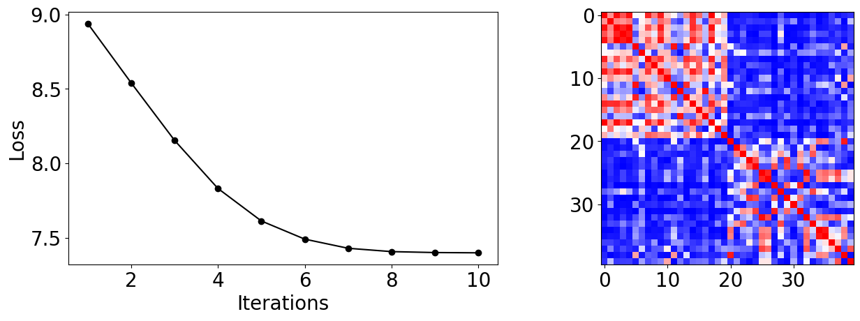
கர்னல் பயிற்சி செயல்முறையை காட்சிப்படுத்தவும்#
From the callback data, we can plot how the loss evolves during the training process. We see it converges rapidly and reaches high test accuracy on this dataset with our choice of inputs.
இறுதி கர்னல் மேட்ரிக்ஸையும் நாம் காட்டலாம், இது பயிற்சி மாதிரிகளுக்கு இடையே உள்ள ஒற்றுமையின் அளவீடு ஆகும்.
[7]:
plot_data = cb_qkt.get_callback_data()  # callback data
K = optimized_kernel.evaluate(X_train)  # kernel matrix evaluated on the training samples

plt.rcParams["font.size"] = 20
fig, ax = plt.subplots(1, 2, figsize=(14, 5))
ax[0].plot([i + 1 for i in range(len(plot_data[0]))], np.array(plot_data[2]), c="k", marker="o")
ax[0].set_xlabel("Iterations")
ax[0].set_ylabel("Loss")
ax[1].imshow(K, cmap=matplotlib.colormaps["bwr"])
fig.tight_layout()
plt.show()
[8]:
import qiskit.tools.jupyter

%qiskit_version_table
%qiskit_copyright
Version Information
| Qiskit Software | Version |
|---|---|
qiskit-terra | 0.25.0 |
qiskit-aer | 0.13.0 |
qiskit-machine-learning | 0.7.0 |
| System information | |
| Python version | 3.8.13 |
| Python compiler | Clang 12.0.0 |
| Python build | default, Oct 19 2022 17:54:22 |
| OS | Darwin |
| CPUs | 10 |
| Memory (Gb) | 64.0 |
| Mon May 29 12:50:08 2023 IST | |
This code is a part of Qiskit
© Copyright IBM 2017, 2023.
This code is licensed under the Apache License, Version 2.0. You may
obtain a copy of this license in the LICENSE.txt file in the root directory
of this source tree or at http://www.apache.org/licenses/LICENSE-2.0.
Any modifications or derivative works of this code must retain this
copyright notice, and modified files need to carry a notice indicating
that they have been altered from the originals.