The Extended Stabilizer Simulator

Introduction

The Extended Simulator is a new method for classically simulating quantum circuits available in the latest release of Qiskit-Aer.

This method is an implementation of the ideas published in the paper Simulation of quantum circuits by low-rank stabilizer decompositions by Bravyi, Browne, Calpin, Campbell, Gosset & Howard, 2018, arXiv:1808.00128.

It uses a different representation of a quantum circuit, that gives it some unique capabilities. This notebook will give some examples of what the extended stabilizer method can do.

For example:

from qiskit import QuantumCircuit, transpile
from qiskit_aer import AerSimulator
from qiskit.tools.visualization import plot_histogram

import random

circ = QuantumCircuit(40, 40)

# Initialize with a Hadamard layer
circ.h(range(40))
# Apply some random CNOT and T gates
qubit_indices = [i for i in range(40)]
for i in range(10):
    control, target, t = random.sample(qubit_indices, 3)
    circ.cx(control, target)
    circ.t(t)
circ.measure(range(40), range(40))

<qiskit.circuit.instructionset.InstructionSet at 0x7fbd18a23310>

We’ve created a random circuit with just 60 gates, that acts on 40 qubits. But, because of the number of qubits, if we wanted to run this with say the statevector simulator then I hope you have access to terabytes of RAM!

# Create statevector method simulator
statevector_simulator = AerSimulator(method='statevector')

# Transpile circuit for backend
tcirc = transpile(circ, statevector_simulator)

# Try and run circuit
statevector_result =  statevector_simulator.run(tcirc, shots=1).result()
print('This succeeded?: {}'.format(statevector_result.success))
print('Why not? {}'.format(statevector_result.status))

Simulation failed and returned the following error message:
ERROR:  [Experiment 0] Insufficient memory to run circuit "circuit-2" using the statevector simulator.

This succeeded?: False
Why not? ERROR:  [Experiment 0] Insufficient memory to run circuit "circuit-2" using the statevector simulator.

The Extended Stabilizer method, in contrast, handles this circuit just fine. (Though it needs a couple of minutes!)

# Create extended stabilizer method simulator
extended_stabilizer_simulator = AerSimulator(method='extended_stabilizer')

# Transpile circuit for backend
tcirc = transpile(circ, extended_stabilizer_simulator)

extended_stabilizer_result = extended_stabilizer_simulator.run(tcirc, shots=1).result()
print('This succeeded?: {}'.format(extended_stabilizer_result.success))

This succeeded?: True

How does this work?

If you’re interested in how exactly we can handle such large circuits, then for a detailed explanation you can read the paper!

For running circuits, however, it’s important to just understand the basics.

The Extended Stabilizer method is made up of two parts. The first is a method of decomposing quantum circuits into stabilizer circuits, a special class of circuit that can be efficiently simulated classically. The second is then a way of combining these circuits to perform measurements.

The number of terms you need scales with the number of what we call non-Clifford Gates. At the moment, the method knows how to handle the following methods:

circ.t(qr[qubit])
circ.tdg(qr[qubit])
circ.ccx(qr[control_1], qr[control_2], qr[target])
circ.u1(rotation_angle, qr[qubit])

The simulator is also able to handle circuits of up to 63 qubits.

One thing that’s important to note is these decompositions are approximate. This means that the results aren’t exactly the same as with the State Vector simulator.

small_circ = QuantumCircuit(2, 2)
small_circ.h(0)
small_circ.cx(0, 1)
small_circ.t(0)
small_circ.measure([0, 1], [0, 1])
# This circuit should give 00 or 11 with equal probability...
expected_results ={'00': 50, '11': 50}

tsmall_circ = transpile(small_circ, extended_stabilizer_simulator)
result = extended_stabilizer_simulator.run(
    tsmall_circ, shots=100).result()
counts = result.get_counts(0)
print('100 shots in {}s'.format(result.time_taken))

100 shots in 0.4958779811859131s

plot_histogram([expected_results, counts],
               legend=['Expected', 'Extended Stabilizer'])

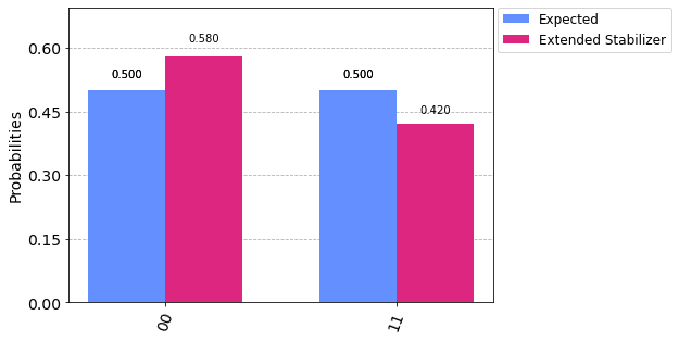
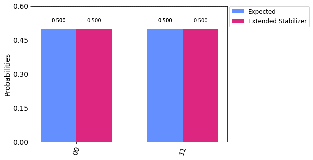
You can control this approximation error using the extended_stabilizer_approximation_error in Qiskit Aer. The default error is 0.05. The smaller the error, the more precise the results, but also the longer your simulation will take and the more memory it will require.

# Add runtime options for extended stabilizer simulator
opts = {'extended_stabilizer_approximation_error': 0.03}

reduced_error = extended_stabilizer_simulator.run(
    tsmall_circ, shots=100, **opts).result()

reduced_error_counts = reduced_error.get_counts(0)
print('100 shots in {}s'.format(reduced_error.time_taken))
plot_histogram([expected_results, reduced_error_counts],
               legend=['Expected', 'Extended Stabilizer'])

100 shots in 1.404871940612793s

Simulator Options

There are several other options you can tweak to control how the extended stabilizer method performs. What these options are and their explanation can all be found in the Qiskit Aer documentation. However, I want to highlight two important ones that can help to optimize your simulations.

To perform measurements, the extended stabilizer method uses a Markov chain method to sample outcomes at random. This Markov chain has to be run for some time we call the ‘mixing time’ before it will start sampling, and has to be re-mixed for every circuit shot.

If you expect your circuit output to be concentrated on just a few output states, then you can likely optimize your simulations by reducing the extended_stabilizer_mixing_time option.

print("The circuit above, with 100 shots at precision 0.03 "
      "and default mixing time, needed {}s".format(int(reduced_error.time_taken)))

opts = {
    'extended_stabilizer_approximation_error': 0.03,
    'extended_stabilizer_mixing_time': 100
}

optimized = extended_stabilizer_simulator.run(
    tsmall_circ, shots=100, **opts).result()

print('Dialing down the mixing time, we completed in just {}s'.format(optimized.time_taken))

The circuit above, with 100 shots at precision 0.03 and default mixing time, needed 1s
Dialing down the mixing time, we completed in just 1.4710919857025146s

Similarly, if your circuit has some non-zero probability on all amplitudes (e.g. if it’s a random circuit), then you can avoid this expensive re-mixing step to take multiple shots from the output at once. This can be enabled by setting extended_stabilizer_measure_sampling=True.

For example, let’s look again at the random circuit from the start of the tutorial, running for 100 shots:

# We set these options here only to make the example run more quickly.
opts = {'extended_stabilizer_mixing_time': 100}

multishot = extended_stabilizer_simulator.run(
    tcirc, shots=100, **opts).result()
print("100 shots took {} s".format(multishot.time_taken))

100 shots took 29.634929895401 s

opts = {
    'extended_stabilizer_measure_sampling': True,
    'extended_stabilizer_mixing_time': 100
}

measure_sampling = extended_stabilizer_simulator.run(
    circ, shots=100, **opts).result()
print("With the optimization, 100 shots took {} s".format(result.time_taken))

With the optimization, 100 shots took 0.4958779811859131 s

When shall I use it?

If you have smaller circuits with lots of non-Clifford gates, then the statevector method will likely perform better than the extended stabilizer. If however you want to look at circuits on many qubits, without needing access to high performance computation, then give this method a try!

import qiskit.tools.jupyter
%qiskit_version_table
%qiskit_copyright

Version Information

Qiskit Software	Version
Qiskit	0.25.0
Terra	0.17.0
Aer	0.8.0
Ignis	0.6.0
Aqua	0.9.0
IBM Q Provider	0.12.2
System information
Python	3.7.7 (default, May 6 2020, 04:59:01) [Clang 4.0.1 (tags/RELEASE_401/final)]
OS	Darwin
CPUs	6
Memory (Gb)	32.0
Fri Apr 02 12:28:14 2021 EDT

This code is a part of Qiskit

© Copyright IBM 2017, 2021.

This code is licensed under the Apache License, Version 2.0. You may
obtain a copy of this license in the LICENSE.txt file in the root directory
of this source tree or at http://www.apache.org/licenses/LICENSE-2.0.

Any modifications or derivative works of this code must retain this
copyright notice, and modified files need to carry a notice indicating
that they have been altered from the originals.