Simulators#
Introduction#
This notebook shows how to import the Qiskit Aer simulator backend and use it to run ideal (noise free).
[4]:
import numpy as np

# Import Qiskit
from qiskit import QuantumCircuit, transpile
from qiskit_aer import AerSimulator
from qiskit.visualization import plot_histogram, plot_state_city
import qiskit.quantum_info as qi
The AerSimulator#
AerSimulator.available_devices(): Return the available simulation devices.AerSimulator.available_methods(): Return the available simulation methods.
[5]:
simulator = AerSimulator()
Simulating a Quantum Circuit#
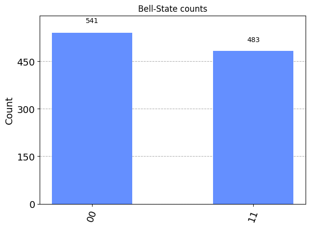
The basic operation runs a quantum circuit and returns a counts dictionary of measurement outcomes. Here we run a simple circuit that prepares a 2-qubit Bell-state \(\left|\psi\right\rangle = \frac{1}{\sqrt{2}}\left(\left|0,0\right\rangle + \left|1,1 \right\rangle\right)\) and measures both qubits.
[6]:
# Create circuit
circ = QuantumCircuit(2)
circ.h(0)
circ.cx(0, 1)
circ.measure_all()

# Transpile for simulator
simulator = AerSimulator()
circ = transpile(circ, simulator)

# Run and get counts
result = simulator.run(circ).result()
counts = result.get_counts(circ)
plot_histogram(counts, title='Bell-State counts')
[6]:
Returning measurement outcomes for each shot#
The Simulator also supports returning a list of measurement outcomes for each individual shot. This is enabled by setting the keyword argument memory=True in the run.
[7]:
# Run and get memory
result = simulator.run(circ, shots=10, memory=True).result()
memory = result.get_memory(circ)
print(memory)
['11', '00', '11', '00', '00', '00', '00', '00', '11', '11']
Aer Simulator Options#
The AerSimulator backend supports a variety of configurable options which can be updated using the set_options method. See the AerSimulator API documentation for additional details.
Simulation Method#
The AerSimulator supports a variety of simulation methods, each of which supports a different set of instructions. The method can be set manually using simulator(method=value) option, or a simulator backend with a preconfigured method can be obtained directly from the AerSimulator
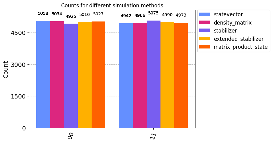
When simulating ideal circuits, changing the method between the exact simulation methods stabilizer, statevector, density_matrix and matrix_product_state should not change the simulation result (other than usual variations from sampling probabilities for measurement outcomes)
Simulation Method Option#
The simulation method is set using the method kwarg. A list supported simulation methods can be returned using available_methods(), these are
"automatic": Default simulation method. Select the simulation method automatically based on the circuit and noise model."statevector": A dense statevector simulation that can sample measurement outcomes from ideal circuits with all measurements at end of the circuit. For noisy simulations each shot samples a randomly sampled noisy circuit from the noise model."density_matrix": A dense density matrix simulation that may sample measurement outcomes from noisy circuits with all measurements at end of the circuit."stabilizer": An efficient Clifford stabilizer state simulator that can simulate noisy Clifford circuits if all errors in the noise model are also Clifford errors."extended_stabilizer": An approximate simulated for Clifford + T circuits based on a state decomposition into ranked-stabilizer state. The number of terms grows with the number of non-Clifford (T) gates."matrix_product_state": A tensor-network statevector simulator that uses a Matrix Product State (MPS) representation for the state. This can be done either with or without truncation of the MPS bond dimensions depending on the simulator options. The default behaviour is no truncation."unitary": A dense unitary matrix simulation of an ideal circuit. This simulates the unitary matrix of the circuit itself rather than the evolution of an initial quantum state. This method can only simulate gates, it does not support measurement, reset, or noise."superop": A dense superoperator matrix simulation of an ideal or noisy circuit. This simulates the superoperator matrix of the circuit itself rather than the evolution of an initial quantum state. This method can simulate ideal and noisy gates, and reset, but does not support measurement.
[9]:
# Increase shots to reduce sampling variance
shots = 10000


# Statevector simulation method
sim_statevector = AerSimulator(method='statevector')
job_statevector = sim_statevector.run(circ, shots=shots)
counts_statevector = job_statevector.result().get_counts(0)

# Stabilizer simulation method
sim_stabilizer = AerSimulator(method='stabilizer')
job_stabilizer = sim_stabilizer.run(circ, shots=shots)
counts_stabilizer = job_stabilizer.result().get_counts(0)


# Extended Stabilizer method
sim_extstabilizer = AerSimulator(method='extended_stabilizer')
job_extstabilizer = sim_extstabilizer.run(circ, shots=shots)
counts_extstabilizer = job_extstabilizer.result().get_counts(0)

# Density Matrix simulation method
sim_density = AerSimulator(method='density_matrix')
job_density = sim_density.run(circ, shots=shots)
counts_density = job_density.result().get_counts(0)

# Matrix Product State simulation method
sim_mps = AerSimulator(method='matrix_product_state')
job_mps = sim_mps.run(circ, shots=shots)
counts_mps = job_mps.result().get_counts(0)


plot_histogram([ counts_statevector,counts_stabilizer ,counts_extstabilizer, counts_density, counts_mps],
               title='Counts for different simulation methods',
               legend=[ 'statevector',
                       'density_matrix','stabilizer','extended_stabilizer', 'matrix_product_state'])
[9]:
Automatic Simulation Method#
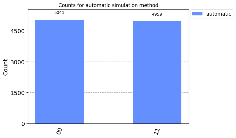
The default simulation method is automatic which will automatically select a one of the other simulation methods for each circuit based on the instructions in those circuits. A fixed simulation method can be specified by by adding the method name when getting the backend, or by setting the method option on the backend.
[10]:
# automatic
sim_automatic = AerSimulator(method='automatic')
job_automatic = sim_automatic.run(circ, shots=shots)
counts_automatic = job_automatic.result().get_counts(0)

plot_histogram([counts_automatic], title='Counts for automatic simulation method',legend=[ 'automatic'])
[10]:
GPU Simulation#
The statevector, density_matrix and unitary simulators support running on a NVidia GPUs. For these methods the simulation device can also be manually set to CPU or GPU using simulator = AerSimmulator(method='statevector',device='GPU') backend option.
[11]:
from qiskit_aer import AerError

# Initialize a GPU backend
# Note that the cloud instance for tutorials does not have a GPU
# so this will raise an exception.
try:
    simulator_gpu = AerSimulator(method='statevector', device='GPU')

except AerError as e:
    print(e)
Installing GPU Support#
In order to install and run the GPU supported simulators on Linux, you need CUDA® 11.2 or newer previously installed. CUDA® itself would require a set of specific GPU drivers. Please follow CUDA® installation procedure in the NVIDIA® web.
If you want to install our GPU supported simulators, you have to install this other package:
pip install qiskit-aer-gpu
The package above is for CUDA® 12, so if your system has CUDA® 11 installed, install separate package:
pip install qiskit-aer-gpu-cu11
This will overwrite your current qiskit-aer package installation giving you the same functionality found in the canonical qiskit-aer package, plus the ability to run the GPU supported simulators: statevector, density matrix, and unitary.
Note: This package is only available on x86_64 Linux. For other platforms that have CUDA support, you will have to build from source. You can refer to the contributing guide for instructions on doing this.
[12]:
from qiskit_aer import AerError

# Initialize a GPU backend
# Note that the cloud instance for tutorials does not have a GPU
# so this will raise an exception.
try:
    simulator_gpu = AerSimulator(method='tensor_network', device='GPU')

except AerError as e:
    print(e)
Simulation Precision#
One of the available simulator options allows setting the float precision for the statevector, density_matrix, unitary and superop methods. This is done using the set_precision="single" or precision="double" (default) option:
[13]:
simulator = AerSimulator(method='statevector')
simulator.set_options(precision='single')

# Run and get counts
result = simulator.run(circ).result()
counts = result.get_counts(circ)
print(counts)
{'00': 505, '11': 519}
Setting the simulation precision applies to both CPU and GPU simulation devices. Single precision will halve the required memory and may provide performance improvements on certain systems.
Custom Simulator Instructions#
Saving the simulator state#
The state of the simulator can be saved in a variety of formats using custom simulator instructions.
Circuit method |
Description |
Supported Methods |
|---|---|---|
|
Save the simulator state in the native format for the simulation method |
All |
|
Save the simulator state as a statevector |
|
|
Save the simulator state as a Clifford stabilizer |
|
|
Save the simulator state as a density matrix |
|
|
Save the simulator state as a a matrix product state tensor |
|
|
Save the simulator state as unitary matrix of the run circuit |
|
|
Save the simulator state as superoperator matrix of the run circuit |
|
Note that these instructions are only supported by the Aer simulator and will result in an error if a circuit containing them is run on a non-simulator backend such as an IBM Quantum device.
Saving the final statevector#
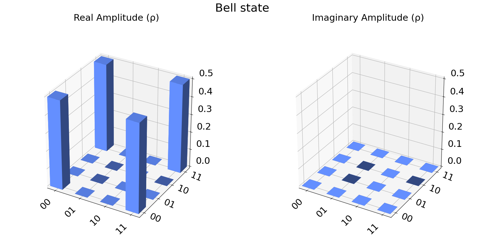
To save the final statevector of the simulation we can append the circuit with the save_statevector instruction. Note that this instruction should be applied before any measurements if we do not want to save the collapsed post-measurement state
[16]:
# Construct quantum circuit without measure
circ = QuantumCircuit(2)
circ.h(0)
circ.cx(0, 1)
circ.save_statevector()

# Transpile for simulator
simulator = AerSimulator(method='statevector')
circ = transpile(circ, simulator)

# Run and get statevector
result = simulator.run(circ).result()
statevector = result.get_statevector(circ)
plot_state_city(statevector, title='Bell state')
[16]:
Saving the circuit unitary#
To save the unitary matrix for a QuantumCircuit we can append the circuit with the save_unitary instruction. Note that this circuit cannot contain any measurements or resets since these instructions are not supported on for the "unitary" simulation method
[17]:
# Construct quantum circuit without measure
circ = QuantumCircuit(2)
circ.h(0)
circ.cx(0, 1)
circ.save_unitary()

# Transpile for simulator
simulator = AerSimulator(method = 'unitary')
circ = transpile(circ, simulator)

# Run and get unitary
result = simulator.run(circ).result()
unitary = result.get_unitary(circ)
print("Circuit unitary:\n", np.asarray(unitary).round(5))
Circuit unitary:
 [[ 0.70711+0.j  0.70711-0.j  0.     +0.j  0.     +0.j]
 [ 0.     +0.j  0.     +0.j  0.70711+0.j -0.70711+0.j]
 [ 0.     +0.j  0.     +0.j  0.70711+0.j  0.70711-0.j]
 [ 0.70711+0.j -0.70711+0.j  0.     +0.j  0.     +0.j]]
Saving multiple states#
We can also apply save instructions at multiple locations in a circuit. Note that when doing this we must provide a unique label for each instruction to retrieve them from the results
[18]:
# Construct quantum circuit without measure
steps = 5
circ = QuantumCircuit(1)
for i in range(steps):
    circ.save_statevector(label=f'psi_{i}')
    circ.rx(i * np.pi / steps, 0)
circ.save_statevector(label=f'psi_{steps}')

# Transpile for simulator
simulator = AerSimulator(method= 'automatic')
circ = transpile(circ, simulator)

# Run and get saved data
result = simulator.run(circ).result()
data = result.data(0)
data
[18]:
{'psi_5': Statevector([-1.+0.00000000e+00j,  0.-5.55111512e-17j],
             dims=(2,)),
 'psi_4': Statevector([-0.30901699+0.j        ,  0.        -0.95105652j],
             dims=(2,)),
 'psi_3': Statevector([0.58778525+0.j        , 0.        -0.80901699j],
             dims=(2,)),
 'psi_2': Statevector([0.95105652+0.j        , 0.        -0.30901699j],
             dims=(2,)),
 'psi_1': Statevector([1.+0.j, 0.+0.j],
             dims=(2,)),
 'psi_0': Statevector([1.+0.j, 0.+0.j],
             dims=(2,))}
Setting the simulator to a custom state#
The AerSimulator allows setting a custom simulator state for several of its simulation methods using custom simulator instructions
Circuit method |
Description |
Supported Methods |
|---|---|---|
|
Set the simulator state to the specified statevector |
|
|
Set the simulator state to the specified Clifford stabilizer |
|
|
Set the simulator state to the specified density matrix |
|
|
Set the simulator state to the specified unitary matrix |
|
|
Set the simulator state to the specified superoperator matrix |
|
Notes: * These instructions must be applied to all qubits in a circuit, otherwise an exception will be raised. * The input state must also be a valid state (statevector, density matrix, unitary etc) otherwise an exception will be raised. * These instructions can be applied at any location in a circuit and will override the current state with the specified one. Any classical register values (e.g. from preceding measurements) will be unaffected * Set state instructions are only supported by the Aer simulator and will result in an error if a circuit containing them is run on a non-simulator backend such as an IBM Quantum device.
Setting a Custom Statevector#
The set_statevector instruction can be used to set a custom Statevector state. The input statevector must be valid (\(|\langle\psi|\psi\rangle|=1\))
[19]:
# Generate a random statevector
num_qubits = 2
psi = qi.random_statevector(2 ** num_qubits, seed=100)

# Set initial state to generated statevector
circ = QuantumCircuit(num_qubits)
circ.set_statevector(psi)
circ.save_state()

# Transpile for simulator
simulator = AerSimulator(method='statevector')
circ = transpile(circ, simulator)

# Run and get saved data
result = simulator.run(circ).result()
result.data(0)
[19]:
{'statevector': Statevector([-0.49859823-0.41410205j,  0.12480824+0.46132192j,
               0.33634191+0.30214216j,  0.234309  +0.3036574j ],
             dims=(2, 2))}
Using the initialize instruction#
It is also possible to initialize the simulator to a custom statevector using the initialize instruction. Unlike the set_statevector instruction this instruction is also supported on real device backends by unrolling to reset and standard gate instructions.
[20]:
# Use initilize instruction to set initial state
circ = QuantumCircuit(num_qubits)
circ.initialize(psi, range(num_qubits))
circ.save_state()

# Transpile for simulator
simulator = AerSimulator(method= 'statevector')
circ = transpile(circ, simulator)

# Run and get result data
result = simulator.run(circ).result()
result.data(0)
[20]:
{'statevector': Statevector([-0.49859823-0.41410205j,  0.12480824+0.46132192j,
               0.33634191+0.30214216j,  0.234309  +0.3036574j ],
             dims=(2, 2))}
Setting a custom density matrix#
The set_density_matrix instruction can be used to set a custom DensityMatrix state. The input density matrix must be valid (\(Tr[\rho]=1, \rho \ge 0\))
[21]:
num_qubits = 2
rho = qi.random_density_matrix(2 ** num_qubits, seed=100)
circ = QuantumCircuit(num_qubits)
circ.set_density_matrix(rho)
circ.save_state()

# Transpile for simulator
simulator = AerSimulator(method='density_matrix')
circ = transpile(circ, simulator)

# Run and get saved data
result = simulator.run(circ).result()
result.data(0)
[21]:
{'density_matrix': DensityMatrix([[ 0.2075308 +0.j        ,  0.13161422-0.01760848j,
                  0.0442826 +0.07742704j,  0.04852053-0.01303171j],
                [ 0.13161422+0.01760848j,  0.20106116+0.j        ,
                  0.02568549-0.03689812j,  0.0482903 -0.04367912j],
                [ 0.0442826 -0.07742704j,  0.02568549+0.03689812j,
                  0.39731492+0.j        , -0.01114025-0.13426423j],
                [ 0.04852053+0.01303171j,  0.0482903 +0.04367912j,
                 -0.01114025+0.13426423j,  0.19409312+0.j        ]],
               dims=(2, 2))}
Setting a custom stabilizer state#
The set_stabilizer instruction can be used to set a custom Clifford stabilizer state. The input stabilizer must be a valid Clifford.
[22]:
# Generate a random Clifford C
num_qubits = 2
stab = qi.random_clifford(num_qubits, seed=100)

# Set initial state to stabilizer state C|0>
circ = QuantumCircuit(num_qubits)
circ.set_stabilizer(stab)
circ.save_state()

# Transpile for simulator
simulator = AerSimulator(method= "stabilizer")
circ = transpile(circ, simulator)

# Run and get saved data
result = simulator.run(circ).result()
result.data(0)
[22]:
{'stabilizer': StabilizerState(['+ZZ', '-IZ'])}
Setting a custom unitary#
The set_unitary instruction can be used to set a custom unitary Operator state. The input unitary matrix must be valid (\(U^\dagger U=\mathbb{1}\))
[23]:
# Generate a random unitary
num_qubits = 2
unitary = qi.random_unitary(2 ** num_qubits, seed=100)

# Set initial state to unitary
circ = QuantumCircuit(num_qubits)
circ.set_unitary(unitary)
circ.save_state()

# Transpile for simulator
simulator = AerSimulator(method='unitary')
circ = transpile(circ, simulator)

# Run and get saved data
result = simulator.run(circ).result()
result.data(0)
[23]:
{'unitary': Operator([[-0.44885724-0.26721573j,  0.10468034-0.00288681j,
             0.4631425 +0.15474915j, -0.11151309-0.68210936j],
           [-0.37279054-0.38484834j,  0.3820592 -0.49653433j,
             0.14132327-0.17428515j,  0.19643043+0.48111423j],
           [ 0.2889092 +0.58750499j,  0.39509694-0.22036424j,
             0.49498355+0.2388685j ,  0.25404989-0.00995706j],
           [ 0.01830684+0.10524311j,  0.62584001+0.01343146j,
            -0.52174025-0.37003296j,  0.12232823-0.41548904j]],
          input_dims=(2, 2), output_dims=(2, 2))}
[37]:
import qiskit
qiskit.__version__
[37]:
'1.0.1'