Note
This page was generated from docs/tutorials/06_qubit_mappers.ipynb.
Mapping to the Qubit Space#
The problems and operators with which you interact in Qiskit Nature (usually) need to be mapped into the qubit space before they can be solved with our quantum algorithms. This task is handled by the various QubitMapper classes.
In this tutorial, you will learn about the various options available to you.
Fermionic Mappers#
This section deals with fermionic mappers, which transform fermionic operators into the qubit space. This is mostly used by the electronic structure stack but also finds application for the `FermiHubbardModel <TODO>`__.
There exist different mapping types with different properties. Qiskit Nature already supports the following fermionic mappings:
Jordan-Wigner (Zeitschrift für Physik, 47, 631-651 (1928))
Parity (The Journal of chemical physics, 137(22), 224109 (2012))
Bravyi-Kitaev (Annals of Physics, 298(1), 210-226 (2002))
We will discuss some of these in the following sections. You should learn all the information necessary, to comfortable work with any of the available mappers.
In order to discuss the various mappings, we will be using the electronic structure Hamiltonian of the H2 molecule. For more information on how to obtain this, please refer to the electronic structure tutorial.
[1]:
from qiskit_nature.second_q.drivers import PySCFDriver

driver = PySCFDriver()
problem = driver.run()
fermionic_op = problem.hamiltonian.second_q_op()
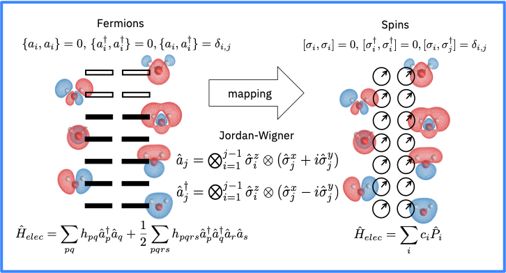
The Jordan-Wigner Mapping#
The Jordan-Wigner mapping is the most straight-forward mapping with the simplest physical interpretation, because it maps the occupation of one spin-orbital to the occupation of one qubit.
You can construct use it like so:
[2]:
from qiskit_nature.second_q.mappers import JordanWignerMapper

mapper = JordanWignerMapper()
[3]:
qubit_jw_op = mapper.map(fermionic_op)
print(qubit_jw_op)
SparsePauliOp(['IIII', 'IIIZ', 'IIZI', 'IIZZ', 'IZII', 'IZIZ', 'ZIII', 'ZIIZ', 'YYYY', 'XXYY', 'YYXX', 'XXXX', 'IZZI', 'ZIZI', 'ZZII'],
              coeffs=[-0.81054798+0.j,  0.17218393+0.j, -0.22575349+0.j,  0.12091263+0.j,
  0.17218393+0.j,  0.16892754+0.j, -0.22575349+0.j,  0.16614543+0.j,
  0.0452328 +0.j,  0.0452328 +0.j,  0.0452328 +0.j,  0.0452328 +0.j,
  0.16614543+0.j,  0.17464343+0.j,  0.12091263+0.j])
The Parity Mapping#
The Parity mapping is the dual mapping to the Jordan-Wigner one, in the sense that it encodes the parity information locally on one qubit, whereas the occupation information is delocalized over all qubits.
[4]:
from qiskit_nature.second_q.mappers import ParityMapper

mapper = ParityMapper()
[5]:
qubit_p_op = mapper.map(fermionic_op)
print(qubit_p_op)
SparsePauliOp(['IIII', 'IIIZ', 'IIZZ', 'IIZI', 'IZZI', 'IZZZ', 'ZZII', 'ZZIZ', 'ZXIX', 'IXZX', 'ZXZX', 'IXIX', 'IZIZ', 'ZZZZ', 'ZIZI'],
              coeffs=[-0.81054798+0.j,  0.17218393+0.j, -0.22575349+0.j,  0.12091263+0.j,
  0.17218393+0.j,  0.16892754+0.j, -0.22575349+0.j,  0.16614543+0.j,
  0.0452328 +0.j, -0.0452328 +0.j, -0.0452328 +0.j,  0.0452328 +0.j,
  0.16614543+0.j,  0.17464343+0.j,  0.12091263+0.j])
This has one major benefit for the case of problems in which we want to preserve the number of particles of each spin species; it allows us to remove 2 qubits, because the information in them becomes redundant. Since Qiskit Nature arranges the qubits in block-order, such that the first half encodes the alpha-spin, and the second half the beta-spin information, this means we can remove the N/2-th and N-th qubit.
To do this, you need to specify the number of particles in your system, like so:
[6]:
mapper = ParityMapper(num_particles=problem.num_particles)
[7]:
qubit_op = mapper.map(fermionic_op)
print(qubit_op)
SparsePauliOp(['II', 'IZ', 'ZI', 'ZZ', 'XX'],
              coeffs=[-1.05237325+0.j,  0.39793742+0.j, -0.39793742+0.j, -0.0112801 +0.j,
  0.1809312 +0.j])
More advanced qubit reductions#
It is also possible to perform more advanced qubit reductions, which are based on finding Z2 symmetries in the Hilbert space of the qubit. A requirement for this to be useful, is that you know in which symmetry-subspace you need to look for your actual solution of interest. This can be a bit tricky, but luckily the problem classes of Qiskit Nature provide you with a utility to automatically determine that correct subspace.
Here is how you can use this to your advantage:
[8]:
tapered_mapper = problem.get_tapered_mapper(mapper)
print(type(tapered_mapper))
<class 'qiskit_nature.second_q.mappers.tapered_qubit_mapper.TaperedQubitMapper'>
[9]:
qubit_op = tapered_mapper.map(fermionic_op)
print(qubit_op)
SparsePauliOp(['I', 'Z', 'X'],
              coeffs=[-1.04109314+0.j, -0.79587485+0.j, -0.1809312 +0.j])
As you can see here, the H2 molecule is such a simple system that we can simulate it entirely on a single qubit!
Interleaved ordering#
As mentioned previously, Qiskit Nature arranges the fermionic spin-up and spin-down parts of the qubit register in block-order. However, sometimes one may want to interleave the registers instead. This can be achieved by means of the InterleavedQubitMapper. This can be shown best upon inspection of the HarteeFock initial state circuit:
[10]:
from qiskit_nature.second_q.circuit.library import HartreeFock
[11]:
hf_state = HartreeFock(2, (1, 1), JordanWignerMapper())
hf_state.draw()
[11]:
     ┌───┐
q_0: ┤ X ├
     └───┘
q_1: ─────
     ┌───┐
q_2: ┤ X ├
     └───┘
q_3: ─────
[12]:
from qiskit_nature.second_q.mappers import InterleavedQubitMapper
[13]:
interleaved_mapper = InterleavedQubitMapper(JordanWignerMapper())
[14]:
hf_state = HartreeFock(2, (1, 1), interleaved_mapper)
hf_state.draw()
[14]:
     ┌───┐
q_0: ┤ X ├
     ├───┤
q_1: ┤ X ├
     └───┘
q_2: ─────

q_3: ─────
[15]:
import tutorial_magics

%qiskit_version_table
%qiskit_copyright
Version Information
| Software | Version |
|---|---|
qiskit | 1.0.1 |
qiskit_algorithms | 0.3.0 |
qiskit_nature | 0.7.2 |
| System information | |
| Python version | 3.8.18 |
| OS | Linux |
| Fri Feb 23 10:25:26 2024 UTC | |
This code is a part of a Qiskit project
© Copyright IBM 2017, 2024.
This code is licensed under the Apache License, Version 2.0. You may
obtain a copy of this license in the LICENSE.txt file in the root directory
of this source tree or at http://www.apache.org/licenses/LICENSE-2.0.
Any modifications or derivative works of this code must retain this
copyright notice, and modified files need to carry a notice indicating
that they have been altered from the originals.