注釈
このページは docs/tutorials/12_deuteron_binding_energy.ipynb から生成されました。
重水素原子核の陽子と中性子の結合エネルギー#
現在の量子コンピューティングでは、量子プロセッサーに誤り訂正符号が実装されていないため、ノイズに悩まされることになります。このノイズが結果に悪影響を及ぼし、その結果、高い信頼性と精度が期待できない場合、現在取り組むことのできる問題が制限される可能性があります。
しかし、重陽子原子核の陽子と中性子の結合エネルギーの計算のように、数量子ビットしか必要としない問題も存在します [1]。この問題は、先に述べた課題にもかかわらず、良い結果を得られるシナリオの一例です。
ステップ 1: 問題に取り組むために必要なパッケージをインポートする#
[1]:
import numpy as np
import matplotlib.pyplot as plt
from IPython.display import display, clear_output
from qiskit.primitives import Estimator
from qiskit_algorithms import VQE
from qiskit_algorithms.observables_evaluator import estimate_observables
from qiskit_algorithms.optimizers import COBYLA, SLSQP
from qiskit.circuit import QuantumCircuit, Parameter
from qiskit.circuit.library import TwoLocal
from qiskit.quantum_info import Pauli, SparsePauliOp
from qiskit.utils import algorithm_globals
from qiskit_nature.second_q.operators import FermionicOp
from qiskit_nature.second_q.mappers import JordanWignerMapper
ステップ 2: いくつかの機能を定義する#
重水素のハミルトニアンの定義を始める前に、クロネッカーデルタを実装したユーティリティー関数を定義する必要があり、それは次のように定義されます。
\(\delta_{n,m} = \bigg\{\begin{array}{c}0, \ \textrm{if} \ n \neq m \\1, \ \textrm{if } \ n = m.\end{array}\).
この関数は [1] で示される重水素のハミルトニアンの定義に登場します。以下に、クロネッカーのデルタ関数を定義するコードの一部を示します。
[2]:
def kronecker_delta_function(n: int, m: int) -> int:
    """An implementation of the Kronecker delta function.

    Args:
        n (int): The first integer argument.
        m (int): The second integer argument.

    Returns:
        Returns 1 if n = m, else returns 0.
    """
    return int(n == m)
[1] では、重水素のハミルトニアンの式は \(H_N = \sum_{n,m=0}^{N-1}\langle m|(T+V)|n\rangle a_{m}^\dagger a_n\) と表されます。ここで \(|n\rangle\) と \(|m\rangle\) は調和振動子基底の量子状態を表し、 \(a_m^\dagger\) と \(a_n\) はそれぞれ生成演算子と消滅演算子を表します。
\(H_N\) を定義するコードを作成するために、運動エネルギーと位置エネルギーの行列要素が必要です。これらの式も [1] で見つけることができます。
\(\langle m|T|n\rangle = \frac{\hbar\omega}{2}\left[\left(2n+\frac{3}{2}\right)\delta_{n,m}-\sqrt{n(n+\frac{1}{2})}\delta_{n,m+1}-\sqrt{(n+1)(n+\frac{3}{2})}\delta_{n,m-1}\right],\) \(\langle m|V|n\rangle = V_0\delta_{n,0}\delta_{n,m}.\)
ここで、 \(V_0 = -5.68658111 \textrm{MeV}\) で、 \(hbaromega = 7 \textrm{MeV}\) です。しかし、このように書かれたハミルトニアンは、量子コンピューターでは直接処理できません。量子コンピューターは、パウリ行列に基づくゲートを通して量子ビットを操作するからです。そこで、生成消滅演算子をパウリ演算子に変換する必要があります。そのために、Jordan-Wigner変換を利用します。
\(a_n^\dagger \ \rightarrow \ \frac{1}{2}\left[\prod_{j=0}^{n-1}-Z_j\right](X_n-iY_n),\)
\(a_n \ \rightarrow \ \frac{1}{2}\left[\prod_{j=0}^{n-1}-Z_j\right](X_n+iY_n).\)
幸い、Qiskit Natureにはフェルミオン演算子を定義し、Jordan-Wigner変換によってこの種の演算子をパウリ演算子に変換するツールがあります。最初に、forループを使ってラベルと係数をタプルに構築し、保存します。この後、タプルをリストに追加します。それぞれの文字列ラベルと係数はハミルトニアンの運動の項 \(\langle m|T|n\rangle\) とポテンシャルの項 \(\langle m|V|n\rangle\) を定義します。forループの最後に、ラベルと係数のタプルを含むリストを FermionicOp に渡して、生成消滅演算子からハミルトニアンを作成する必要があります。このハミルトニアンをパウリ演算子で書き換える必要があります。そのためには、 JordanWignerMapper() を使用します。Qiskit Natureツールに関するより詳しい情報は、Qiskit Natureドキュメント [2] を読むことをお勧めします。
[3]:
def create_deuteron_hamiltonian(
    N: int, hbar_omega: float = 7.0, V_0: float = -5.68658111
) -> SparsePauliOp:
    """Creates a version of the Deuteron Hamiltonian as a qubit operator.

    Args:
        N (int): An integer number that represents the dimension of the
            basis.
        hbar_omega (float, optional): The value of the product of hbar and omega. Defaults to 7.0.
        V_0 (float, optional): The value of the potential energy. Defaults to -5.68658111.

    Returns:
        SparsePauliOp: The qubit-space Hamiltonian that represents the Deuteron.
    """
    hamiltonian_terms = {}
    for m in range(N):
        for n in range(N):

            label = "+_{} -_{}".format(str(n), str(m))
            coefficient_kinect = (hbar_omega / 2) * (
                (2 * n + 3 / 2) * kronecker_delta_function(n, m)
                - np.sqrt(n * (n + (1 / 2))) * kronecker_delta_function(n, m + 1)
                - np.sqrt((n + 1) * (n + (3 / 2)) * kronecker_delta_function(n, m - 1))
            )
            hamiltonian_terms[label] = coefficient_kinect

            coefficient_potential = (
                V_0 * kronecker_delta_function(n, 0) * kronecker_delta_function(n, m)
            )
            hamiltonian_terms[label] += coefficient_potential

    hamiltonian = FermionicOp(hamiltonian_terms, num_spin_orbitals=N)
    mapper = JordanWignerMapper()
    qubit_hamiltonian = mapper.map(hamiltonian)
    if not isinstance(qubit_hamiltonian, SparsePauliOp):
        qubit_hamiltonian = qubit_hamiltonian.primitive

    return qubit_hamiltonian
さて、Qiskit Natureのツールを使って、パウリ演算子でハミルトニアンを構築する方法がわかりました。しかし、これで終わりではありません。パラメーター化された量子回路を通してansatzを構築し、 VQE を使用して重水素のハミルトニアンの最小固有値 (結合エネルギー) を計算します。
ステップ 3: Qiskit ツールを使用して、重水素原子核の陽子と中性子の結合エネルギーを計算する#
前のステップで重水素原子核の陽子と中性子の結合エネルギーの計算に役立つ機能を定義しました。 今度は、私たちが構築したツールを使って問題を解決するプロセスを始める時です。
重水素のハミルトニアン( \(N = 1\) )の最も単純な形である \(H_1\) から始めましょう。[1] では、著者らは \(N = 1,2,3\) の基底状態のエネルギーを計算し、その値を使ってエネルギーを外挿し、重水素の基底状態のエネルギーの値である \(-2.22 \MeV\) に到達しようと試みています。ここでは、ハミルトニアン \(H_1\), \(H_2\), \(H_3\), \(H_4\) を格納するリストを作成します。なぜなら、これらのハミルトニアンは後に基底状態を計算するために使用することになるからです。これを行うには、上で定義した create_deuteron_hamiltonian という関数でリスト内包を行います。
[4]:
deuteron_hamiltonians = [create_deuteron_hamiltonian(i) for i in range(1, 5)]
参考文献 [1] に、N = 1, 2, 3 の大きさの重水素のハミルトニアンの厳密な式が示されています。
\(H_1 = 0.218291(Z_0-I_0)\)
\(H_2 = 5.906709I_1\otimes I_0 + 0.218291I_1\otimes Z_0 - 6.215Z_1\otimes I_0 - 2.143304(X_1\otimes X_0 + Y_1 \otimes Y_0)\)
\(H_3 = I_2\otimes H_2 + 9.625(I_2\otimes I_1\otimes I_0 - Z_2\otimes I_1\otimes I_0) - 3.913119(X_2\otimes X_1\otimes I_0 + Y_2\otimes Y_1\otimes I_0)\)
もし、 create_deuteron_hamiltonian が正しい結果を与えているかどうかを知りたければ、上に示した式と比較する必要があります。この目的のために、関数 create_deuteron_hamiltonian によって生成されたハミルトニアンを以下のセルに記載しました。
[5]:
for i, hamiltonian in enumerate(deuteron_hamiltonians):
    print("Deuteron Hamiltonian: H_{}".format(i + 1))
    print(hamiltonian)
    print("\n")
Deuteron Hamiltonian: H_1
SparsePauliOp(['I', 'Z'],
              coeffs=[-0.21829055+0.j,  0.21829055+0.j])


Deuteron Hamiltonian: H_2
SparsePauliOp(['II', 'IZ', 'XX', 'YY', 'ZI'],
              coeffs=[ 5.90670945+0.j,  0.21829055+0.j, -2.14330352+0.j, -2.14330352+0.j,
 -6.125     +0.j])


Deuteron Hamiltonian: H_3
SparsePauliOp(['III', 'IIZ', 'IXX', 'IYY', 'IZI', 'XXI', 'YYI', 'ZII'],
              coeffs=[15.53170945+0.j,  0.21829055+0.j, -2.14330352+0.j, -2.14330352+0.j,
 -6.125     +0.j, -3.91311896+0.j, -3.91311896+0.j, -9.625     +0.j])


Deuteron Hamiltonian: H_4
SparsePauliOp(['IIII', 'IIIZ', 'IIXX', 'IIYY', 'IIZI', 'IXXI', 'IYYI', 'IZII', 'XXII', 'YYII', 'ZIII'],
              coeffs=[ 28.65670945+0.j,   0.21829055+0.j,  -2.14330352+0.j,  -2.14330352+0.j,
  -6.125     +0.j,  -3.91311896+0.j,  -3.91311896+0.j,  -9.625     +0.j,
  -5.67064811+0.j,  -5.67064811+0.j, -13.125     +0.j])
検証の結果、この関数は \(H_1\), \(H_2\), \(H_3\) に対して正しい結果を与えていることがわかります。 [1] には \(H_4\) の式がありませんが、帰納法により、以前の結果が [1] で与えられた式と一致すれば、その結果は正しいに違いないと言うことは可能です。
[1] では、著者らは実量子デバイスで計算をしたかったので、Depthの浅いansatzで作業をしました。この量子回路は [1] で見ることができます。このチュートリアルの冒頭で述べたように、現在利用可能な量子ハードウェアは、量子エラー訂正が実装されておらず、ノイズが多いため、良い結果を得るためには浅いDepthの量子回路で動作させる必要があります。
下のコードセルで示されているように、 Parameter() を使用して [1] で紹介されている回路を構築するために、 \(\theta\) (theta) と \(\eta\) (eta) という2つのパラメーターを定義する必要があります。
[6]:
theta = Parameter(r"$\theta$")
eta = Parameter(r"$\eta$")
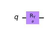
`[1] <https://arxiv.org/pdf/1801.03897.pdf>`__で示される回路を構築する指示に従うと、上記で定義されたパラメーターを使用して以下の回路を得られます。
[7]:
wavefunction = QuantumCircuit(1)
wavefunction.ry(theta, 0)
wavefunction.draw("mpl")
[7]:
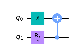
[8]:
wavefunction2 = QuantumCircuit(2)
wavefunction2.x(0)
wavefunction2.ry(theta, 1)
wavefunction2.cx(1, 0)
wavefunction2.draw("mpl")
[8]:
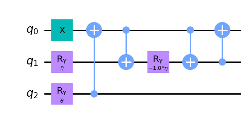
[9]:
wavefunction3 = QuantumCircuit(3)
wavefunction3.x(0)
wavefunction3.ry(eta, 1)
wavefunction3.ry(theta, 2)
wavefunction3.cx(2, 0)
wavefunction3.cx(0, 1)
wavefunction3.ry(-eta, 1)
wavefunction3.cx(0, 1)
wavefunction3.cx(1, 0)
wavefunction3.draw("mpl")
[9]:
残念ながら、[1] では \(H_4\) のansatzのための浅い回路を見つけることができません。よって、今のところ \(N = 4\) を扱いませんが、後でansatzとして TwoLocal を使ってこの問題に戻りましょう。
これらの回路をテストの構成のためにansatzリストに格納します。
[10]:
ansatz = [wavefunction, wavefunction2, wavefunction3]
生成された演算子のサイズが小さいので、 \(H_1\), :math: H_2, \(H_3\), :math:`H_4`の結合エネルギーを得るとき、ハミルトニアン行列の最小固有値を見つけるプロセスにnumpy関数 (古典的なメソッド) を使うことができます。このタスクは、以下のコードセルの for ループで実行されます。
[11]:
reference_values = []
print("Exact binding energies calculated through numpy.linalg.eigh \n")
for i, hamiltonian in enumerate(deuteron_hamiltonians):
    eigenvalues, eigenstates = np.linalg.eigh(hamiltonian.to_matrix())
    reference_values.append(eigenvalues[0])
    print("Exact binding energy for H_{}: {}".format(i + 1, eigenvalues[0]))
Exact binding energies calculated through numpy.linalg.eigh

Exact binding energy for H_1: -0.43658110999999966
Exact binding energy for H_2: -1.7491598763215301
Exact binding energy for H_3: -2.045670898406441
Exact binding energy for H_4: -2.143981030799862
上記の結果を参照値として使用します。 したがって、Estimatorが良い結果をもたらすかどうかを確認するためにそれらを使用できます。 以下のコードセルでは、Estimatorと SLSQP オプティマイザーを使用して、ansatz と ハミルトニアンのペアに対して VQE アルゴリズムを実行しました。
[12]:
print(
    "Results using Estimator for H_1, H_2 and H_3 with the ansatz given in the reference paper \n"
)
for i in range(3):
    seed = 42
    algorithm_globals.random_seed = seed
    vqe = VQE(Estimator(), ansatz=ansatz[i], optimizer=SLSQP())
    vqe_result = vqe.compute_minimum_eigenvalue(deuteron_hamiltonians[i])
    binding_energy = vqe_result.optimal_value
    print("Binding energy for H_{}: {} MeV".format(i + 1, binding_energy))
Results using Estimator for H_1, H_2 and H_3 with the ansatz given in the reference paper

Binding energy for H_1: -0.4365811096105766 MeV
Binding energy for H_2: -1.7491595316575452 MeV
Binding energy for H_3: -2.045670898257444 MeV
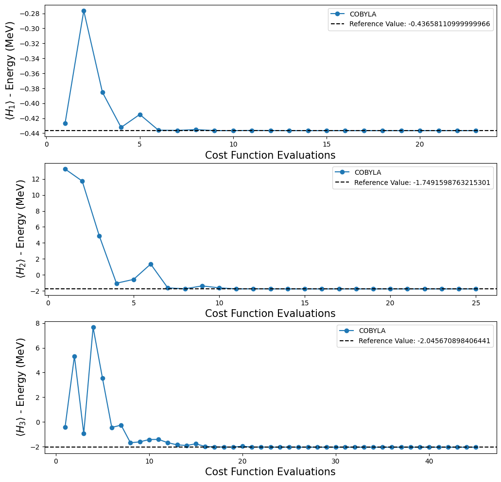
我々の結果は古典的な手法で得られた基準値と一致していることがわかります。また、Qiskitで提供されているオプティマイザーのオプションもどれが良いかテストしました。そのために、VQE の callback オプションを使用し、カウントと値のリストを保存できるようにしました。この情報を使って、オプティマイザーが参照値に収束するかどうか、収束する場合はどのくらいの速度で収束するかをプロットすることが可能です。しかし、以下のコードセルでは、簡単のために COBYLA オプティマイザーのみを使用しています。
[13]:
def callback(eval_count, parameters, mean, std):
    # Overwrites the same line when printing
    display("Evaluation: {}, Energy: {}, Std: {}".format(eval_count, mean, std))
    clear_output(wait=True)
    counts.append(eval_count)
    values.append(mean)
    params.append(parameters)
    deviation.append(std)
[14]:
plots = []

for i in range(3):

    counts = []
    values = []
    params = []
    deviation = []
    seed = 42
    algorithm_globals.random_seed = seed
    vqe = VQE(Estimator(), ansatz=ansatz[i], optimizer=COBYLA(), callback=callback)
    vqe_result = vqe.compute_minimum_eigenvalue(deuteron_hamiltonians[i])
    plots.append([counts, values])
'Evaluation: 45, Energy: -2.045670636012936, Std: {}'
前のコードセルで VQE を実行して取得した結果をプロットします。
[15]:
fig, ax = plt.subplots(nrows=3, ncols=1)
fig.set_size_inches((12, 12))
for i, plot in enumerate(plots):
    ax[i].plot(plot[0], plot[1], "o-", label="COBYLA")
    ax[i].axhline(
        y=reference_values[i],
        color="k",
        linestyle="--",
        label=f"Reference Value: {reference_values[i]}",
    )
    ax[i].legend()
    ax[i].set_xlabel("Cost Function Evaluations", fontsize=15)
    ax[i].set_ylabel(r"$\langle H_{} \rangle$ - Energy (MeV)".format(i + 1), fontsize=15)
plt.show()
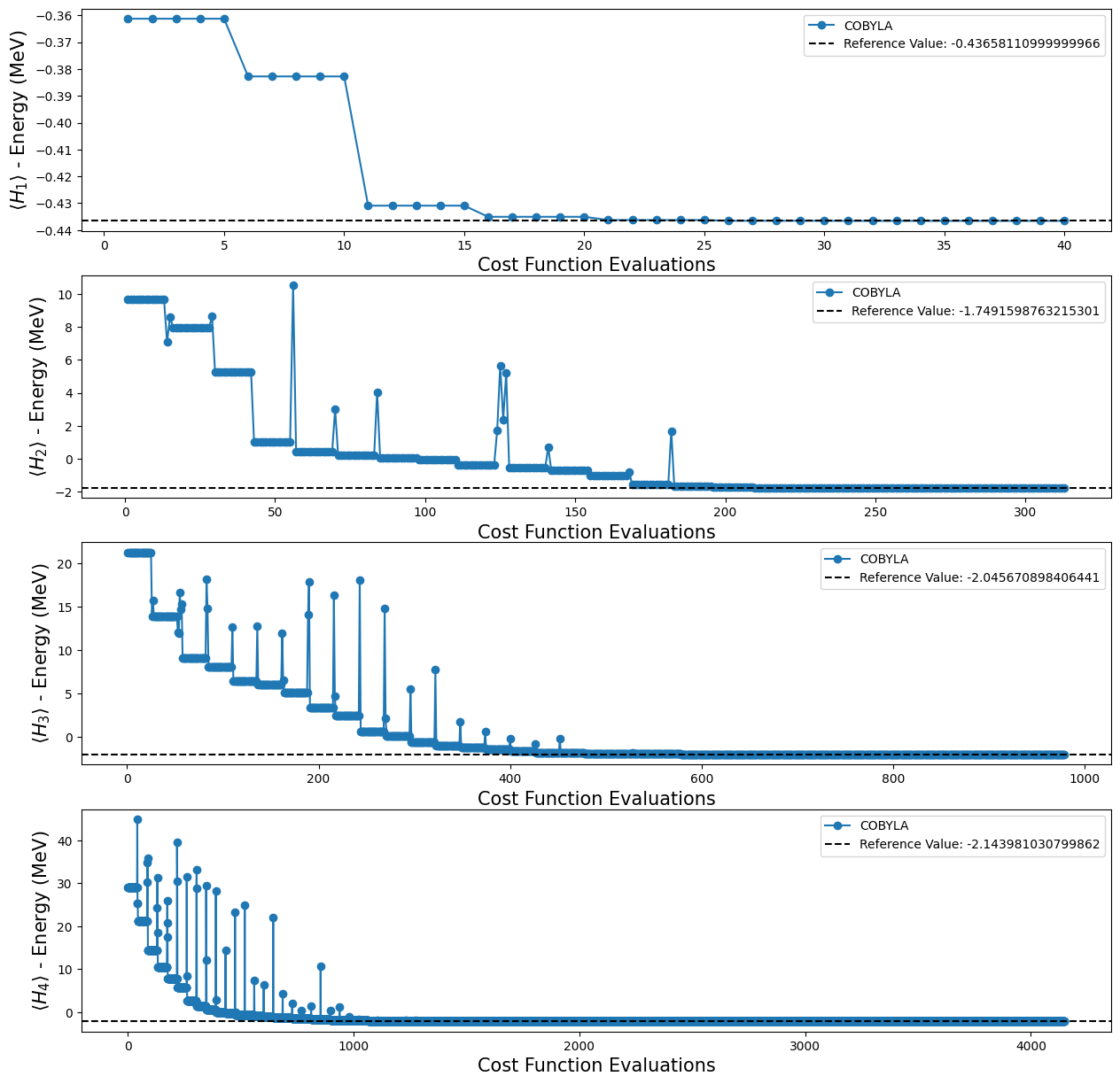
[1] で示した量子回路では、 \(H_4\) の参照値に到達できるかどうかをテストすることができません。なぜなら、前述のように、このハミルトニアンの ansatz がないためです。幸いなことに、Qiskitには ansatz を作成する関数がいくつか用意されているので、実験が終わってしまうわけではありません。我々の目的のための新しい ansatz を作るためにTwoLocal関数を使うことにしました。以下のコードでは、forループを使って各ハミルトニアンの TwoLocal ansatzを含むリストを作成しています。
[16]:
twolocal_ansatzes = []
for i in range(1, 5):
    ansatz = TwoLocal(
        deuteron_hamiltonians[i - 1].num_qubits,
        ["rz", "ry"],
        "cx",
        entanglement="full",
        reps=i,
        initial_state=None,
    )
    twolocal_ansatzes.append(ansatz)
新しいタイプの ansatz で、古典的な手法で得られた参照値に到達できるかどうかを確認できます。 この検証を行うには、以前に行った実験を繰り返す必要がありますが、今度は、TwoLocal 関数を使用して定義された ansatz を使用します。
[17]:
print("Results using Estimator for H_1, H_2, H_3 and H_4 with TwoLocal ansatz \n")
seed = 42
algorithm_globals.random_seed = seed
for i in range(4):
    vqe = VQE(Estimator(), ansatz=twolocal_ansatzes[i], optimizer=SLSQP())
    vqe_result = vqe.compute_minimum_eigenvalue(deuteron_hamiltonians[i])
    binding_energy = vqe_result.optimal_value
    print("Binding energy for H_{}:".format(i + 1), binding_energy, "MeV")
Results using Estimator for H_1, H_2, H_3 and H_4 with TwoLocal ansatz

Binding energy for H_1: -0.4365806560191138 MeV
Binding energy for H_2: -1.7491598681936242 MeV
Binding energy for H_3: -2.045670763548605 MeV
Binding energy for H_4: -2.1439130048015045 MeV
[18]:
seed = 42
algorithm_globals.random_seed = seed

plots_tl = []
for i in range(4):

    counts = []
    values = []
    params = []
    deviation = []
    vqe = VQE(
        Estimator(),
        ansatz=twolocal_ansatzes[i],
        optimizer=SLSQP(),
        callback=callback,
    )
    vqe_result = vqe.compute_minimum_eigenvalue(deuteron_hamiltonians[i])
    plots_tl.append([counts, values])
'Evaluation: 4149, Energy: -2.143913004801629, Std: {}'
4 つの TwoLocal ansatz を使用して、以下の結果を得ました:
[19]:
fig, ax = plt.subplots(nrows=4, ncols=1)
fig.set_size_inches((15, 15))
for i, plot in enumerate(plots_tl):
    ax[i].plot(plot[0], plot[1], "o-", label="COBYLA")
    ax[i].axhline(
        y=reference_values[i],
        color="k",
        linestyle="--",
        label=f"Reference Value: {reference_values[i]}",
    )
    ax[i].legend()
    ax[i].set_xlabel("Cost Function Evaluations", fontsize=15)
    ax[i].set_ylabel(r"$\langle H_{} \rangle$ - Energy (MeV)".format(i + 1), fontsize=15)
plt.show()
ステップ 4: 観測量の期待値を計算する#
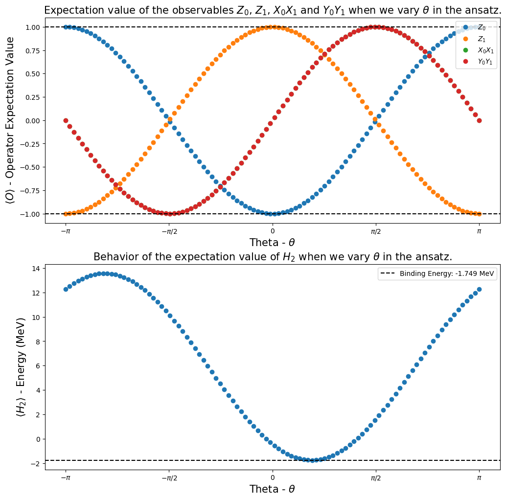
Qiskit Advocate Mentorship Program プロジェクトにおける我々の目標の一つは、興味のあるいくつかの観測量の期待値を計算可能であることを示し、 ansatz 回路のパラメーターを変えたときにそれらがどう振る舞うかを示すことでした。我々の場合、興味のある観測量は \(I_1 \otimes Z_0\), \(Z_1 \otimes I_0\), \(X_1 \otimes X_0\), \(Y_1 \otimes Y_0\) と \(H_2\) で、さらにパラメーター \(\theta\) を区間 \([-\pi,\pi]\) 以内で変化させた時のそれらの動作を調査しています。
ディラック記法 (ブラケット) では、観測値の期待値の定義 \(\hat{O}\) は [3] [4] に等しくなります。
\(\langle \hat{O} \rangle_\psi = \langle \psi(\vec{\theta})|\hat{O}|\psi(\vec{\theta}) \rangle\).
以下のコードは、観測値の期待値を計算する関数を定義しています。 パラメーター化された量子回路と、これらのパラメーター(角度) の値を持つリストが与えられます。
[20]:
def calculate_observables_exp_values(
    quantum_circuit: QuantumCircuit, observables: list, angles: list
) -> list:
    """Calculate the expectation value of an observable given the quantum
    circuit that represents the wavefunction and a list of parameters.

        Args:
            quantum_circuit (QuantumCircuit): A parameterized quantum circuit
            that represents the wavefunction of the system.

            observables (list): A list containing the observables that we want
            to know the expectation values.

            angles (list): A list with the values that will be used in the
            'bind_parameters' method.

        Returns:
            list_exp_values (list): A list containing the expectation values
            of the observables given as input.
    """
    list_exp_values = []
    for observable in observables:
        exp_values = []
        for angle in angles:
            qc = quantum_circuit.bind_parameters({theta: angle})
            result = estimate_observables(
                Estimator(),
                quantum_state=qc,
                observables=[observable],
            )

            exp_values.append(result[0][0])
        list_exp_values.append(exp_values)

    return list_exp_values
上記で定義した関数を使用して、関心のある観測量の期待値を計算します。
[21]:
angles = list(np.linspace(-np.pi, np.pi, 100))
observables = [
    Pauli("IZ"),
    Pauli("ZI"),
    Pauli("XX"),
    Pauli("YY"),
    deuteron_hamiltonians[1],
]
h2_observables_exp_values = calculate_observables_exp_values(wavefunction2, observables, angles)
(ステップ2で定義した) 関数 calculate_observables_exp_values を使用して、以下のプロットを得ました。 [1] の結果を再現できていることを示しました。
[22]:
fig, ax = plt.subplots(nrows=2, ncols=1)
fig.set_size_inches((12, 12))
ax[0].plot(angles, h2_observables_exp_values[0], "o", label=r"$Z_0$")
ax[0].plot(angles, h2_observables_exp_values[1], "o", label=r"$Z_1$")
ax[0].plot(angles, h2_observables_exp_values[2], "o", label=r"$X_0X_1$")
ax[0].plot(angles, h2_observables_exp_values[3], "o", label=r"$Y_0Y_1$")
ax[0].axhline(
    y=1,
    color="k",
    linestyle="--",
)
ax[0].axhline(y=-1, color="k", linestyle="--")
ax[0].legend()
ax[0].set_xlabel(r"Theta - $\theta$", fontsize=15)
ax[0].set_ylabel(r"$\langle O \rangle $ - Operator Expectation Value", fontsize=15)
ax[0].set_xticks(
    [-np.pi, -np.pi / 2, 0, np.pi / 2, np.pi],
    labels=[r"$-\pi$", r"$-\pi/2$", "0", r"$\pi/2$", r"$\pi$"],
)
ax[0].set_title(
    r"Expectation value of the observables $Z_0$, $Z_1$, $X_0X_1$ and $Y_0Y_1$ when we vary $\theta$ in the ansatz.",
    fontsize=15,
)
ax[1].plot(angles, h2_observables_exp_values[4], "o")
ax[1].axhline(
    y=reference_values[1],
    color="k",
    linestyle="--",
    label="Binding Energy: {} MeV".format(np.round(reference_values[1], 3)),
)
ax[1].legend()
ax[1].set_xlabel(r"Theta - $\theta$", fontsize=15)
ax[1].set_ylabel(r"$\langle H_2 \rangle $ - Energy (MeV)", fontsize=15)
ax[1].set_xticks(
    [-np.pi, -np.pi / 2, 0, np.pi / 2, np.pi],
    labels=[r"$-\pi$", r"$-\pi/2$", "0", r"$\pi/2$", r"$\pi$"],
)
ax[1].set_title(
    r"Behavior of the expectation value of $H_2$ when we vary $\theta$ in the ansatz.", fontsize=15
)

plt.show()
謝辞#
Qiskit Advocate Mentorship Program 2021 - Fallの期間中に行ったミーティングでのSteve Wood、Soham Pal、Siddhartha Moralesに感謝します。彼らはこのチュートリアルの構築に非常に重要でした。
参考文献#
[1] Dumitrescu, Eugene F., et al. “Cloud quantum computing of an atomic nucleus.” Physical review letters 120.21 (2018): 210501. Arxiv version: https://arxiv.org/pdf/1801.03897.pdf
[2] QisKit Nature Documentation. https://qiskit.org/documentation/nature/
[3] Feynman, R. P., Robert B. Leighton, and Matthew Sands. “The Feynman Lectures on Physics, Volume III: Quantum Mechanics, vol. 3.” (2010). https://www.feynmanlectures.caltech.edu/III_toc.html
[4] 期待値 (量子力学) Wikipedia の記事 https://en.wikipedia.org/wiki/Expectation_value_(quantum_mechanics)
[23]:
import qiskit.tools.jupyter

%qiskit_version_table
%qiskit_copyright
Version Information
| Qiskit Software | Version |
|---|---|
qiskit-terra | 0.24.0.dev0+2b3686f |
qiskit-aer | 0.11.2 |
qiskit-ibmq-provider | 0.19.2 |
qiskit-nature | 0.6.0 |
| System information | |
| Python version | 3.9.16 |
| Python compiler | GCC 12.2.1 20221121 (Red Hat 12.2.1-4) |
| Python build | main, Dec 7 2022 00:00:00 |
| OS | Linux |
| CPUs | 8 |
| Memory (Gb) | 62.50002670288086 |
| Thu Apr 06 09:19:48 2023 CEST | |
This code is a part of Qiskit
© Copyright IBM 2017, 2023.
This code is licensed under the Apache License, Version 2.0. You may
obtain a copy of this license in the LICENSE.txt file in the root directory
of this source tree or at http://www.apache.org/licenses/LICENSE-2.0.
Any modifications or derivative works of this code must retain this
copyright notice, and modified files need to carry a notice indicating
that they have been altered from the originals.